blogs
Get the latest latest breakthroughs from the BCI and neuroscience innovation world.
BCI Kickstarter #01 : Introduction to Brain-Computer Interfaces
Welcome to the first installment of our crash course on Brain-Computer Interfaces (BCIs)! This fascinating field holds immense potential for revolutionizing how we interact with technology and the world around us. In this series, we'll delve into the core concepts, methodologies, and applications of BCIs, providing you with a solid foundation to understand this exciting domain.
What is a BCI?
Brain-Computer Interfaces, or BCIs, are systems that establish a direct communication pathway between the brain and external devices. They bypass traditional neuromuscular pathways, allowing individuals to control machines or receive sensory feedback using only their brain activity. This groundbreaking technology has far-reaching implications for various fields, including healthcare, assistive technology, gaming, and even art.
At its core, a BCI system operates through three fundamental steps:
- Brain Signal Acquisition: Neural activity is recorded using various techniques, such as electroencephalography (EEG), electrocorticography (ECoG), or invasive electrode implants.
- Signal Processing: The acquired brain signals are processed and analyzed to extract meaningful patterns and features related to the user's intent or mental state.
- Output and Control: The extracted information is translated into commands that control external devices, such as prosthetic limbs, wheelchairs, or computer cursors.
BCIs offer a powerful means of communication and control, particularly for individuals with severe motor impairments or those suffering from locked-in syndrome. They open up a world of possibilities for restoring lost function, enhancing human capabilities, and even creating entirely new forms of human-computer interaction.
The Evolution of BCI over time
The history of brain-computer interfaces (BCIs) dates back to 1924 when Hans Berger first recorded human brain activity using electroencephalography (EEG). However, significant BCI research gained momentum in the 1970s at the University of California, Los Angeles (UCLA), focusing on using EEG signals for basic device control. Since then, advancements in the field have propelled BCI technology forward, including:
- Improved Electrodes and Sensors: Development of high-density electrode arrays and more sensitive sensors for better signal acquisition.
- Advanced Signal Processing Techniques: Sophisticated algorithms for filtering noise, artifact removal, and feature extraction from brain signals.
- Machine Learning Revolution: Application of machine learning algorithms for pattern recognition and classification, enabling more accurate decoding of user intent.
These advancements have led to impressive applications of BCIs:
- Restoring Lost Function: Controlling prosthetic limbs, wheelchairs, and communication devices for individuals with paralysis or locked-in syndrome.
- Assistive Technology: Developing tools for environmental control, such as controlling lights or appliances with brain signals.
- Gaming and Entertainment: Creating immersive and interactive experiences using brain-controlled interfaces.
- Neurofeedback and Therapy: Utilizing BCIs for treating conditions like ADHD, anxiety, and chronic pain.
- Cognitive Enhancement: Exploring the potential of BCIs for improving memory, attention, and other cognitive functions.
The future of BCIs is brimming with possibilities. As research progresses, we can expect even more groundbreaking applications that will further transform how we interact with the world and push the boundaries of human potential.
A Look at Different BCI Types
BCI systems are categorized based on their level of invasiveness, each with its own trade-offs in terms of signal quality, complexity, and risk. The three main types are:
Invasive BCI: Direct Access to the Source
Invasive BCIs involve surgically implanting electrodes directly into the brain tissue. This method offers the highest signal quality and allows for the most precise control. However, it also carries the highest risk of medical complications and requires significant expertise for implantation and maintenance.
Example: The Utah Array, a microelectrode array, is a prominent example of an invasive BCI used in research and clinical trials.
Applications: Primarily used for restoring lost motor function in individuals with paralysis or locked-in syndrome, enabling them to control prosthetic limbs, wheelchairs, and communication devices.
Semi-Invasive BCI (ECoG): Bridging the Gap
Semi-invasive BCIs, specifically Electrocorticography (ECoG), involve placing electrodes on the surface of the brain, beneath the skull. This approach offers a balance between signal quality and invasiveness, providing higher resolution than non-invasive methods while minimizing the risks associated with penetrating the brain tissue.
One notable company in this field is Synchron, which employs a minimally invasive endovascular procedure—similar to stent placement—to avoid open brain surgery. Their innovative approach allows for the safe and effective placement of electrodes, enabling patients to interact with technology using their thoughts. In a recent clinical trial, their first participant successfully connected with his wife by digitally controlling his computer through thought.
Applications: ECoG-based BCIs, including those developed by Synchron, are currently used in research settings for investigating brain function and exploring potential applications in epilepsy treatment and motor rehabilitation.
Non-Invasive BCIs: Exploring the Brain from the Outside
Non-invasive BCIs are the most common and accessible type, as they rely on external sensors to record brain activity without the need for surgery. These methods are generally safer and more comfortable for the user. However, the signal quality can be affected by noise and artifacts, requiring sophisticated signal processing techniques for accurate interpretation.
Examples:
- Electroencephalography (EEG): Measures electrical activity in the brain using electrodes placed on the scalp.
- Magnetoencephalography (MEG): Detects magnetic fields generated by brain activity.
- Functional Magnetic Resonance Imaging (fMRI): Measures brain activity by detecting changes in blood flow.
- Functional Near-Infrared Spectroscopy (fNIRS): Measures brain activity by monitoring changes in blood oxygenation
EEG-Based BCIs: A Deep Dive
Among the various non-invasive BCI approaches, electroencephalography (EEG) stands out as a particularly promising and widely adopted technology. EEG-based BCIs leverage the electrical activity generated by the brain, recorded through electrodes placed on the scalp. This method offers several key advantages:
High Temporal Resolution: EEG boasts excellent temporal resolution, capturing brain activity changes in milliseconds. This rapid sampling rate allows for real-time detection of subtle shifts in brain states, crucial for accurate and responsive BCI control.
Portability and Ease of Use: EEG systems are relatively portable and easy to set up, making them suitable for a variety of environments, from research labs to home settings. The non-invasive nature of EEG also contributes to its ease of use, as it doesn't require surgery or complex procedures.
Cost-Effectiveness: Compared to other neuroimaging techniques like fMRI or MEG, EEG is significantly more affordable. This accessibility makes it an attractive option for research, development, and widespread adoption of BCI technology.
Wide Range of Applications: EEG-based BCIs have demonstrated their versatility in a multitude of applications, including:
- Motor Imagery BCIs: Allow users to control devices by imagining specific movements.
- P300 Spellers: Enable users to spell words by focusing their attention on specific letters.
- Steady-State Visual Evoked Potential (SSVEP) BCIs: Utilize visual stimuli to elicit brain responses for control.
- Neurofeedback and Therapy: Provide real-time feedback on brain activity to help users learn to self-regulate their brain states for therapeutic purposes.
Addressing the Limitations:
The primary challenge lies in EEG’s lower spatial resolution compared to invasive or semi-invasive techniques. The electrical signals recorded by EEG electrodes are a mixture of activity from various brain regions, making it more difficult to pinpoint the precise source of the signal. However, advancements in signal processing and machine learning algorithms are continually improving the ability to extract meaningful information from EEG data, mitigating this limitation.
On the whole, EEG-based BCIs, especially when combined with fNIRS, offer a compelling mix of high temporal resolution, portability, affordability, and versatility. This combination enhances the ability to capture both electrical activity and hemodynamic responses in the brain, providing a more comprehensive understanding of brain function. These advantages have propelled EEG to the forefront of BCI research and development, driving innovation and expanding the potential applications of this transformative technology.
The Future is Brain-Powered
Brain-computer interfaces have emerged as a revolutionary technology with the potential to fundamentally change how we interact with the world around us. While various approaches exist, EEG-based BCIs stand out due to their unique combination of high temporal resolution, portability, cost-effectiveness, and versatility. From restoring lost motor function to enhancing cognitive abilities, the applications of EEG-based BCIs are vast and rapidly expanding.
As research and development continue to advance, we can expect even more groundbreaking innovations in the field of BCIs, leading to a future where our brains can seamlessly interact with technology, unlocking new possibilities for communication, control, and human potential.
Ready to Dive Deeper?
This concludes the first part of our crash course on Brain-Computer Interfaces. We've explored the fundamental concepts, different types of BCIs, and the advantages of EEG-based systems.
In the next installments of this series, we'll concern ourselves with specific aspects of BCI technology, covering topics such as:
- Fundamentals of Neuroscience for BCI: Understanding the brain's electrical activity and how it relates to BCI control.
- EEG Signal Acquisition and Processing: Exploring the techniques used to record and analyze EEG data.
- BCI Paradigms and Applications: Examining different types of BCI systems and their specific applications.
- Building Your Own BCI with Python: A hands-on guide to developing your own BCI applications.
Stay tuned for the next exciting chapter in our BCI journey!
BCI Kickstarter #02: Fundamentals of Neuroscience for BCI
Welcome back to our BCI crash course! In the previous blog, we explored the basics of BCIs and different approaches to decoding brain signals. Today, we will explore the fascinating world of neuroscience to understand the foundation upon which these incredible technologies are built. This blog will focus on the electrical activity of the brain, particularly relevant for EEG-based BCIs. By understanding how neurons communicate and generate the rhythmic oscillations that EEG measures, we can gain valuable insights into the development and application of BCI systems.
Basic Brain Anatomy and Function: Your Brain's Control Center
The brain, the most complex organ in the human body, is the command center for our thoughts, emotions, and actions. To understand how BCIs tap into this intricate network, let's explore some key anatomical structures and their functions.
Brain Divisions: A Three-Part Harmony
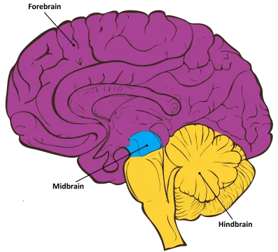
The brain is broadly divided into three main sections:
- Forebrain: The largest and most evolved part of the brain, the forebrain is responsible for higher-level cognitive functions like language, reasoning, and problem-solving. It also processes sensory information from our environment, controls voluntary movement, and regulates emotions and motivations.
- Midbrain: Situated between the forebrain and hindbrain, the midbrain plays a crucial role in relaying sensory information to higher brain centers. It's also involved in motor control, particularly for eye movements, and in regulating sleep-wake cycles and arousal.
- Hindbrain: The oldest and most primitive part of the brain, the hindbrain is responsible for controlling vital autonomic functions such as breathing, heart rate, and blood pressure. It also coordinates balance and movement.
For BCI applications, the forebrain, particularly the cerebrum, is of primary interest. This is where conscious thought, decision-making, and voluntary actions originate.
Cerebral Cortex: The Brain's Outer Layer
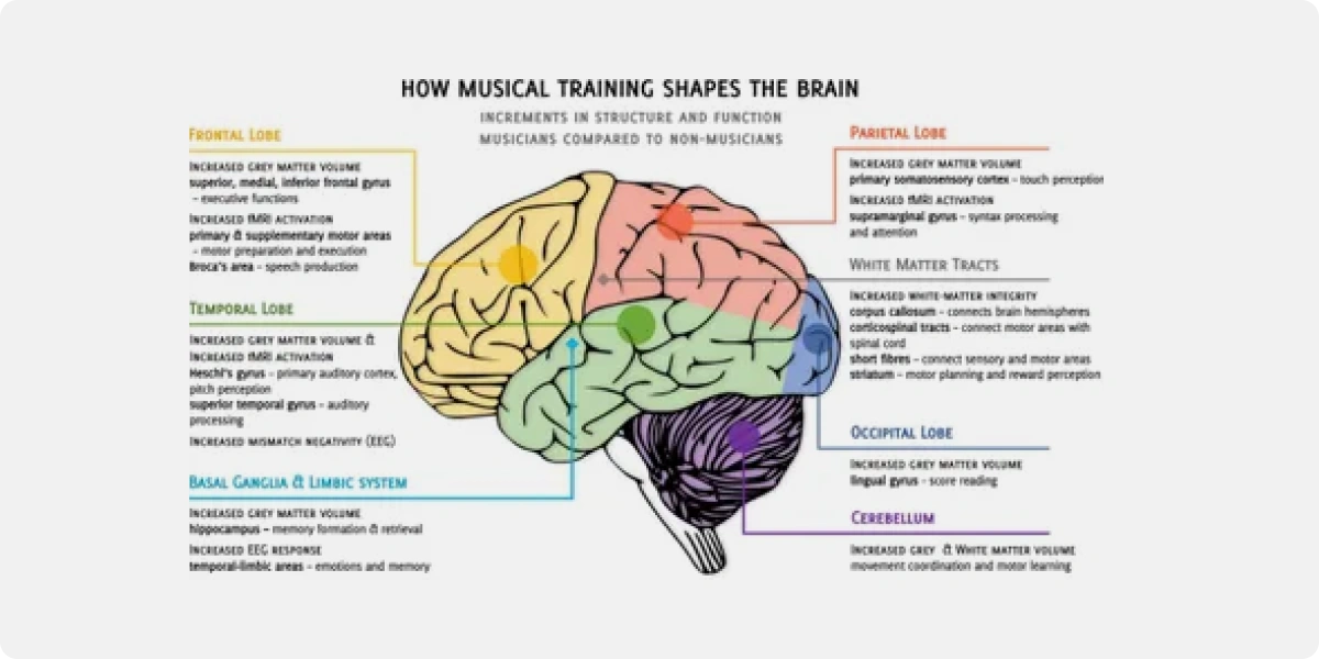
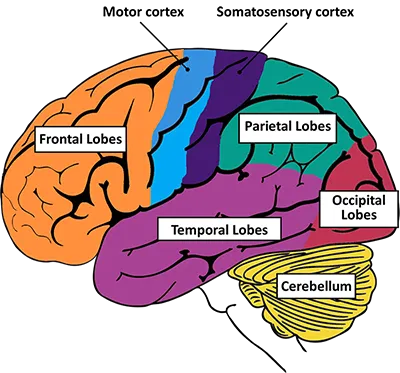
The cerebrum's outer layer, the cerebral cortex, is a wrinkled sheet of neural tissue responsible for many of our higher cognitive abilities. It's divided into four lobes, each with specialized functions:
- Frontal Lobe: The "executive center" of the brain, the frontal lobe is responsible for planning, decision-making, working memory, and voluntary movement. It plays a crucial role in higher-level cognitive functions like reasoning, problem-solving, and language production. Damage to the frontal lobe can impair these functions and lead to changes in personality and behavior.
- Parietal Lobe: The parietal lobe processes sensory information related to touch, temperature, pain, and spatial awareness. It also integrates sensory input from different modalities, helping us form a coherent perception of our surroundings. Damage to the parietal lobe can cause difficulties with spatial navigation, object recognition, and body awareness.
- Temporal Lobe: The temporal lobe is involved in auditory processing, language comprehension, and memory formation. It contains structures like the hippocampus, crucial for long-term memory, and the amygdala, involved in processing emotions, particularly fear and aggression. Damage to the temporal lobe can impair memory, language comprehension, and emotional processing.
- Occipital Lobe: Located at the back of the brain, the occipital lobe is dedicated to visual processing. It receives input from the eyes and interprets visual information, allowing us to perceive shapes, colors, and motion. Damage to the occipital lobe can lead to visual impairments, including blindness or difficulty recognizing objects.
Gray and White Matter: The Brain's Building Blocks
The brain is composed of two main types of tissue:
- Gray Matter: Gray matter gets its color from the densely packed cell bodies of neurons. It is primarily involved in processing information, making decisions, and controlling actions. Gray matter is found in the cerebral cortex, basal ganglia, thalamus, and other brain regions involved in higher-level cognitive functions.
- White Matter: White matter is composed of myelinated axons, the long, slender projections of neurons that transmit electrical signals. Myelin, a fatty substance, acts as an insulator, allowing signals to travel faster and more efficiently. White matter forms the "wiring" that connects different brain regions, enabling communication and coordination between them.
Neural Signaling and Brain Rhythms: The Electrical Symphony of Your Brain
To understand how EEG-based BCIs work, we need to dive deeper into how neurons communicate and generate the electrical signals that EEG measures. This intricate process involves a complex interplay of electrical impulses, chemical messengers, and rhythmic oscillations.
Neurons and Synapses: The Building Blocks of Communication
Neurons are specialized cells that transmit information throughout the nervous system. They have a unique structure:
- Dendrites: Branch-like extensions that receive signals from other neurons.
- Cell Body (Soma): Contains the nucleus and other cellular machinery.
- Axon: A long, slender fiber that transmits electrical signals away from the cell body.
- Synapse: A small gap between the axon of one neuron and the dendrite of another, where communication occurs.
Electrical Signaling: The Language of Neurons
Neurons communicate using electrical impulses called action potentials. These brief, rapid changes in electrical charge travel down the axon, triggered by a complex interplay of ion channels that regulate the flow of charged particles across the neuron's membrane.
Think of an action potential like a wave traveling down a rope. It's an all-or-nothing event; once triggered, it propagates down the axon at a constant speed and amplitude.
When an action potential reaches the synapse, it triggers the release of neurotransmitters, chemical messengers that cross the synaptic gap and bind to receptors on the receiving neuron. This binding can either excite or inhibit the receiving neuron, modulating its likelihood of firing its own action potential.
Neurotransmitters and Receptors: Fine-Tuning the Signals
Neurotransmitters are the brain's chemical messengers, playing a crucial role in regulating mood, cognition, and behavior. Here are some key neurotransmitters relevant to BCI applications:
- Glutamate: The primary excitatory neurotransmitter in the brain, involved in learning, memory, and synaptic plasticity.
- GABA (Gamma-Aminobutyric Acid): The primary inhibitory neurotransmitter, important for calming neural activity and preventing overexcitation.
- Dopamine: Involved in reward, motivation, and motor control, playing a crucial role in Parkinson's disease.
- Acetylcholine: Plays a vital role in muscle contraction, memory, and attention.
Each neurotransmitter binds to specific receptors on the receiving neuron, triggering a cascade of intracellular events that ultimately modulate the neuron's electrical activity.
EEG Rhythms and Oscillations: Decoding the Brain's Rhythms
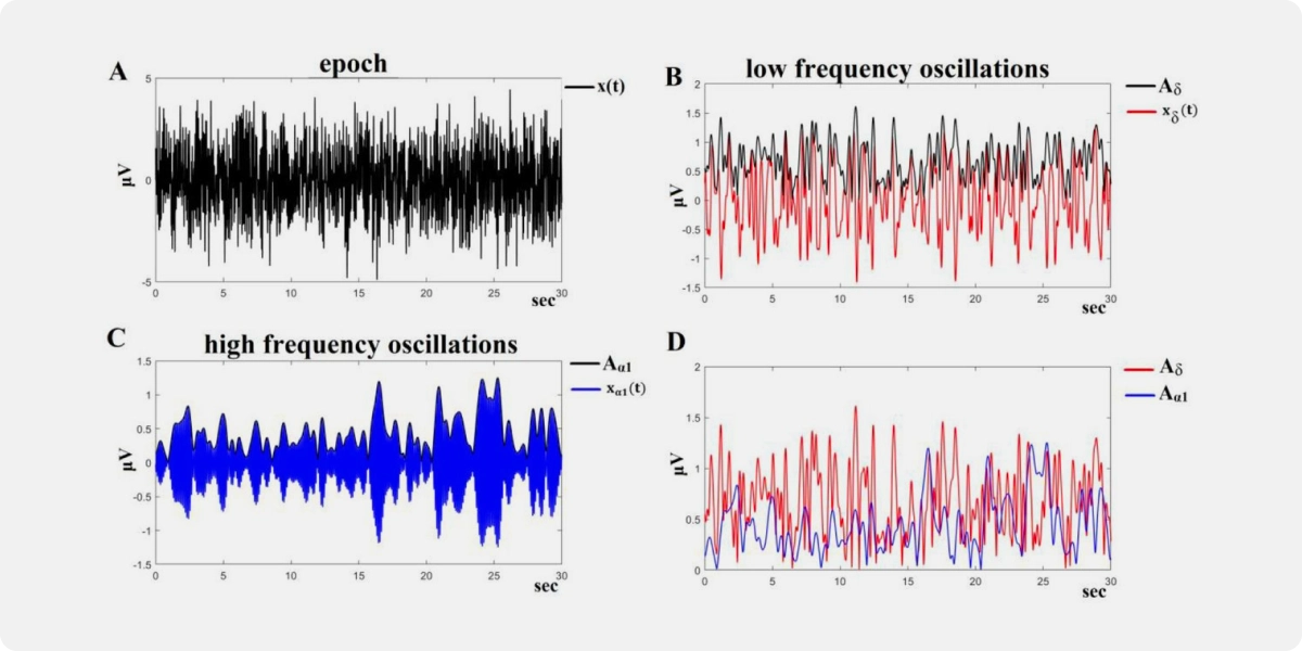
EEG measures the synchronized electrical activity of large groups of neurons firing together, generating rhythmic oscillations that reflect different brain states. These oscillations are categorized into frequency bands:
- Delta (1-4 Hz): The slowest brainwaves, dominant during deep sleep and associated with memory consolidation.
- Theta (4-8 Hz): Prominent during drowsiness, meditation, and creative states, often linked to cognitive processing and working memory.
- Alpha (8-12 Hz): Associated with relaxed wakefulness, particularly with eyes closed. Alpha waves are suppressed during mental exertion and visual processing.
- Beta (12-30 Hz): Reflect active thinking, focus, and alertness. Increased beta activity is observed during tasks requiring sustained attention and cognitive effort.
- Gamma (30-100 Hz): The fastest brainwaves, associated with higher cognitive functions, sensory binding, and conscious awareness.
By analyzing these rhythmic patterns, EEG-based BCIs can decode user intent, mental states, and even diagnose neurological conditions.
Electroencephalography (EEG) and its Significance in BCI: Capturing the Brain's Electrical Whispers
EEG, as we've mentioned throughout this post, is a powerful tool for capturing the electrical activity of the brain, making it a cornerstone of many BCI systems. Let's explore how EEG works and why it's so valuable for decoding brain signals.
How EEG Works: Recording the Brain's Electrical Symphony
EEG measures the electrical potentials generated by synchronized neuronal activity in the cerebral cortex. This is achieved using electrodes placed on the scalp, which detect the tiny voltage fluctuations produced by these electrical currents.
The electrodes are typically arranged according to the 10-20 system, a standardized placement system that ensures consistent and comparable recordings across different individuals and research studies.
The 10-20 System: A Standardized Map for EEG Recording
The 10-20 system is the internationally standardized method for placing EEG electrodes. It provides a consistent framework for recording and interpreting EEG data, allowing researchers and clinicians worldwide to communicate and compare results effectively.
The system is based on specific anatomical landmarks on the skull:
- Nasion: The indentation at the top of the nose, between the eyebrows.
- Inion: The bony prominence at the back of the head.
- Preauricular Points: The depressions just in front of each ear.
Electrodes are placed at intervals of 10% or 20% of the total distance between these reference points, forming a grid-like pattern that covers the scalp.
Each electrode is labeled with a letter and a number:
- Letters: Represent the underlying brain region (Fp for prefrontal, F for frontal, C for central, P for parietal, T for temporal, O for occipital).
- Numbers: Indicate the hemisphere (odd numbers for the left, even numbers for the right, and z for midline).
This standardized system ensures that electrodes are consistently placed in the same locations across different individuals, facilitating reliable comparisons and analysis of EEG data.
High-Density vs. Low-Density Systems: A Matter of Resolution
EEG systems vary in the number of electrodes they use, ranging from a few electrodes in consumer-grade headsets to hundreds of electrodes in research-grade systems.
- High-Density Systems: Provide higher spatial resolution, allowing for more precise localization of brain activity. They are commonly used in research settings for investigating complex cognitive processes and mapping brain function.
- Low-Density Systems: Offer portability and affordability, making them suitable for consumer applications like neurofeedback, meditation training, and sleep monitoring. However, their lower spatial resolution limits their ability to pinpoint specific brain regions.
The choice of system depends on the specific application and the desired level of detail in capturing brain activity.
Types of EEG Electrodes: From Wet to Dry
Various types of EEG electrodes are available, each with its own advantages and disadvantages:
- Wet Electrodes: Require a conductive gel or paste to enhance electrical contact with the scalp. They generally provide better signal quality but can be more time-consuming to apply.
- Dry Electrodes: Don't require conductive gel, making them more convenient and user-friendly, but they might have slightly lower signal quality.
EEG Montages: Choosing Your Viewpoint
EEG montages refer to the way electrode pairs are connected to create the electrical signals displayed. Different montages highlight different aspects of brain activity and can influence the interpretation of EEG data.
Common montages include:
- Bipolar Montage: Each channel represents the voltage difference between two adjacent electrodes, emphasizing localized activity and minimizing the influence of distant sources.
- Referential Montage: Each channel represents the voltage difference between an active electrode and a common reference electrode (e.g., linked mastoids, average reference). This montage provides a broader view of brain activity across regions but can be more susceptible to artifacts from the reference electrode.
The choice of montage depends on the research question or BCI application. Bipolar montages are often preferred for studying localized brain activity, while referential montages are useful for examining activity across broader brain regions.
Further Reading and Resources:
- Principles of Neural Science – Kandel et al
- HarvardX: Fundamentals of Neuroscience, Part 1: The Electrical Properties of the Neuron (https://www.edx.org/learn/neuroscience/harvard-university-fundamentals-of-neuroscience-part-1-the-electrical-properties-of-the-neuron)
- HarvardX: Fundamentals of Neuroscience, Part 2: Neurons and Networks (https://www.edx.org/learn/neuroscience/harvard-university-fundamentals-of-neuroscience-part-2-neurons-and-networks)
- HarvardX: Fundamentals of Neuroscience, Part 3: The Brain (https://www.edx.org/learn/neuroscience/harvard-university-fundamentals-of-neuroscience-part-3-the-brain)
Ready to Dive Deeper into EEG Signal Processing?
This concludes our exploration of the fundamentals of neuroscience for BCI. In the next post, we'll dive into the practical aspects of EEG signal acquisition and processing, exploring the techniques used to extract meaningful information from the raw EEG data.
Stay tuned for our next BCI adventure!
BCI Kickstarter #03: EEG Signal Acquisition and Processing
Welcome back to our BCI crash course! In the previous blog, we explored the basic concepts of BCIs and delved into the fundamentals of neuroscience. Now, it's time to get our hands dirty with the practical aspects of EEG signal acquisition and processing. This blog will guide you through the journey of transforming raw EEG data into a format suitable for meaningful analysis and BCI applications. We will cover signal preprocessing techniques, and feature extraction methods, providing you with the essential tools for decoding the brain's electrical secrets.
Signal Preprocessing Techniques: Cleaning Up the Data
Raw EEG data, fresh from the electrodes, is often a noisy and complex landscape. To extract meaningful insights and develop reliable BCIs, we need to apply various signal preprocessing techniques to clean up the data, remove artifacts, and enhance the true brain signals.
Why Preprocessing is Necessary: Navigating a Sea of Noise
The journey from raw EEG recordings to usable data is fraught with challenges:
- Noise and Artifacts Contamination: EEG signals are susceptible to various sources of interference, both biological (e.g., muscle activity, eye blinks, heartbeats) and environmental (e.g., power line noise, electrode movement). These artifacts can obscure the true brain signals we are interested in.
- Separating True Brain Signals: Even in the absence of obvious artifacts, raw EEG data contains a mix of neural activity related to various cognitive processes. Preprocessing helps us isolate the specific signals relevant to our research or BCI application.
Importing Data: Laying the Foundation
Before we can begin preprocessing, we need to import our EEG data into a suitable software environment. Common EEG data formats include:
- FIF (Functional Imaging File Format): A widely used format developed for MEG and EEG data, supported by the MNE library in Python.
- EDF (European Data Format): Another standard format, often used for clinical EEG recordings.
Libraries like MNE provide functions for reading and manipulating these formats, enabling us to work with EEG data in a programmatic way.
Removing Bad Channels and Interpolation: Dealing with Faulty Sensors
Sometimes, EEG recordings contain bad channels — electrodes that are malfunctioning, poorly placed, or picking up excessive noise. We need to identify and address these bad channels before proceeding with further analysis.
Identifying Bad Channels:
- Visual Inspection: Plotting the raw EEG data and visually identifying channels with unusually high noise levels, flat lines, or other anomalies.
- Automated Methods: Using algorithms that detect statistically significant deviations from expected signal characteristics.
Interpolation:
If a bad channel cannot be salvaged, we can use interpolation to estimate its missing data based on the surrounding good channels. Spherical spline interpolation is a common technique that projects electrode locations onto a sphere and uses a mathematical model to estimate the missing values.
Filtering: Tuning into the Right Frequencies
Filtering is a fundamental preprocessing step that allows us to remove unwanted frequencies from our EEG signal. Different types of filters serve distinct purposes:
- High-Pass Filtering: Removes slow drifts and DC offsets, which are often caused by electrode movement or skin potentials. A typical cutoff frequency for high-pass filtering is around 0.1 Hz.
- Low-Pass Filtering: Removes high-frequency noise, which can originate from muscle activity or electrical interference. A common cutoff frequency for low-pass filtering is around 30 Hz for most cognitive tasks, though some applications may use higher cutoffs for studying gamma activity.
- Band-Pass Filtering: Combines high-pass and low-pass filtering to isolate a specific frequency band of interest, such as the alpha (8-12 Hz) or beta (12-30 Hz) band.
- Notch Filtering: Removes a narrow band of frequencies, typically used to eliminate power line noise (50/60 Hz) or other specific interference.
Choosing the appropriate filter settings is crucial for isolating the relevant brain signals and minimizing the impact of noise on our analysis.
Downsampling: Reducing the Data Load
Downsampling refers to reducing the sampling rate of our EEG signal, which can be beneficial for:
- Reducing data storage requirements: Lower sampling rates result in smaller file sizes.
- Improving computational efficiency: Processing lower-resolution data requires less computing power.
However, we need to be cautious when downsampling to avoid losing important information. The Nyquist-Shannon sampling theorem dictates that we must sample at a rate at least twice the highest frequency of interest in our signal to avoid aliasing, where high frequencies are incorrectly represented as lower frequencies.
Decimation is a common downsampling technique that combines low-pass filtering with sample rate reduction to ensure that we don't introduce aliasing artifacts into our data.
Re-Referencing: Choosing Your Point of View
In EEG recording, each electrode's voltage is measured relative to a reference electrode. The choice of reference can significantly influence the interpretation of our signals, as it affects the baseline against which brain activity is measured.
Common reference choices include:
- Linked Mastoids: Averaging the signals from the mastoid electrodes behind each ear.
- Average Reference: Averaging the signals from all electrodes.
- Other References: Specific electrodes (e.g., Cz) or combinations of electrodes can be chosen based on the research question or BCI application.
Re-referencing allows us to change the reference of our EEG data after it's been recorded. This can be useful for comparing data recorded with different reference schemes or for exploring the impact of different references on signal interpretation. Libraries like MNE provide functions for easily re-referencing data.
Feature Extraction Methods: Finding the Signal in the Noise
Once we've preprocessed our EEG data, it's time to extract meaningful information that can be used for analysis or to train BCI systems. Feature extraction is the process of transforming the preprocessed EEG signal into a set of representative features that capture the essential patterns and characteristics of the underlying brain activity.
What is Feature Extraction? Simplifying the Data Landscape
Raw EEG data, even after preprocessing, is often high-dimensional and complex. Feature extraction serves several important purposes:
- Reducing Data Dimensionality: By extracting a smaller set of representative features, we simplify the data, making it more manageable for analysis and machine learning algorithms.
- Highlighting Relevant Patterns: Feature extraction methods focus on specific aspects of the EEG signal that are most relevant to the research question or BCI application, enhancing the signal-to-noise ratio and improving the accuracy of our analyses.
Time-Domain Features: Analyzing Signal Fluctuations
Time-domain features capture the temporal characteristics of the EEG signal, focusing on how the voltage changes over time. Some common time-domain features include:
- Amplitude:
- Peak-to-Peak Amplitude: The difference between the highest and lowest voltage values within a specific time window.
- Mean Amplitude: The average voltage value over a given time period.
- Variance: A measure of how much the signal fluctuates around its mean value.
- Peak-to-Peak Amplitude: The difference between the highest and lowest voltage values within a specific time window.
- Latency:
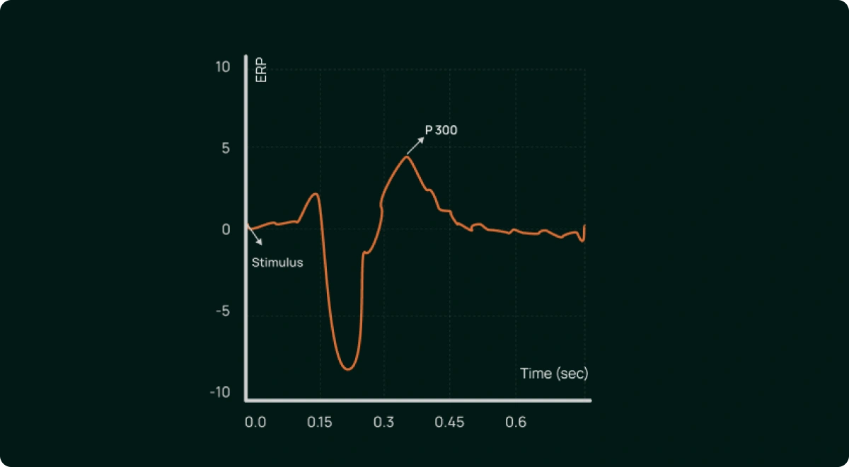
- Onset Latency: The time it takes for a specific event-related potential (ERP) component to appear after a stimulus.
- Peak Latency: The time point at which an ERP component reaches its maximum amplitude.
- Onset Latency: The time it takes for a specific event-related potential (ERP) component to appear after a stimulus.
- Time-Series Analysis:
- Autoregressive Models: Statistical models that predict future values of the signal based on its past values, capturing temporal dependencies in the data.
- Moving Averages: Smoothing techniques that calculate the average of the signal over a sliding window, reducing noise and highlighting trends.
- Autoregressive Models: Statistical models that predict future values of the signal based on its past values, capturing temporal dependencies in the data.
Frequency-Domain Features: Unveiling the Brain's Rhythms
Frequency-domain features analyze the EEG signal in the frequency domain, revealing the power distribution across different frequency bands. Key frequency-domain features include:
- Power Spectral Density (PSD): A measure of the signal's power at different frequencies. PSD is typically calculated using the Fast Fourier Transform (FFT), which decomposes the signal into its constituent frequencies.
- Band Power: The total power within a specific frequency band, such as delta, theta, alpha, beta, or gamma. Band power features are often used in BCI systems to decode mental states or user intent.
Time-Frequency Features: Bridging the Time and Frequency Divide
Time-frequency features provide a combined view of the EEG signal in both time and frequency domains, capturing dynamic changes in frequency content over time. Important time-frequency features include:
- Wavelet Transform: A powerful technique that decomposes the signal into a set of wavelets, functions that vary in both frequency and time duration. Wavelet transforms excel at capturing transient events and analyzing signals with non-stationary frequency content.
- Short-Time Fourier Transform (STFT): Divides the signal into short segments and calculates the FFT for each segment, providing a time-varying spectrum. STFT is useful for analyzing how the frequency content of the signal changes over time.
From Raw Signals to Actionable Insights
The journey from raw EEG data to meaningful insights and BCI control involves a carefully orchestrated sequence of signal acquisition, preprocessing, and feature extraction. Each step plays a crucial role in revealing the hidden patterns within the brain's electrical symphony, allowing us to decode mental states, control external devices, and unlock new possibilities for human-computer interaction.
By mastering these techniques, we can transform the complex and noisy world of EEG recordings into a rich source of information, paving the way for innovative BCI applications that can improve lives and expand our understanding of the human brain.
Further Reading and Resources
- Book: Analyzing Neural Time Series Data: Theory and Practice
By: Mike X Cohen
https://doi.org/10.7551/mitpress/9609.001.0001
ISBN (electronic): 9780262319553
- Tutorial: MNE-Python documentation on preprocessing: https://mne.tools/stable/auto_tutorials/preprocessing/index.html
- Article: Urigüen, J. A., & Garcia-Zapirain, B. (2015). EEG artifact removal—state-of-the-art and guidelines. Journal of Neural Engineering, 12(3), 031001.
What's Next: Real-World BCIs using Signal Processing
This concludes our exploration of EEG signal acquisition and processing. Now that we've learned how to clean up and extract meaningful features from raw EEG data, we are ready to explore how these techniques are used to build real-world BCI applications.
In the next post, we'll dive into the fascinating world of BCI paradigms and applications, discovering the diverse ways BCIs are being used to translate brain signals into actions. Stay tuned!
BCI Kickstarter #04 : Python for BCI: Getting Started
Welcome back to our BCI crash course! We've journeyed through the fundamental concepts of BCIs, delved into the intricacies of the brain, and explored the art of processing raw EEG signals. Now, it's time to empower ourselves with the tools to build our own BCI applications. Python, a versatile and powerful programming language, has become a popular choice for BCI development due to its rich ecosystem of scientific libraries, ease of use, and strong community support. In this post, we'll set up our Python environment and introduce the essential libraries that will serve as our BCI toolkit.
Setting Up Your Python BCI Development Environment: Building Your BCI Lab
Before we can start coding, we need to lay a solid foundation by setting up our Python BCI development environment. This involves choosing the right Python distribution, managing packages, and selecting an IDE that suits our workflow.
Choosing the Right Python Distribution: Anaconda for BCI Experimentation
While several Python distributions exist, Anaconda stands out as a particularly strong contender for BCI development. Here's why:
- Ease of Use: Anaconda simplifies package management and environment creation, streamlining your workflow.
- Conda Package Manager: Conda provides a powerful command-line interface for installing, updating, and managing packages, ensuring you have the right tools for your BCI projects.
- Pre-installed Scientific Libraries: Anaconda comes bundled with essential scientific libraries like NumPy, SciPy, Matplotlib, and Jupyter Notebooks, eliminating the need for separate installations.
You can download Anaconda for free from https://www.anaconda.com/products/distribution.
Managing Packages with Conda: Your BCI Arsenal
Conda, the package manager included with Anaconda, will be our trusty sidekick for managing the libraries and dependencies essential for our BCI endeavors. Here are some key commands:
- Installing Packages: To install a specific package, use the command conda install <package_name>. For example, to install the MNE library for EEG analysis, you would run conda install -c conda-forge mne.
- Creating Environments: Environments allow you to isolate different projects and their dependencies, preventing conflicts between packages. To create a new environment, use the command conda create -n <environment_name> python=<version>. For example, to create an environment named "bci_env" with Python 3.8, you'd run conda create -n bci_env python=3.8.
- Activating Environments: To activate an environment and make its packages available, use the command conda activate <environment_name>. For our "bci_env" example, we'd run conda activate bci_env.
Essential IDEs (Integrated Development Environments): Your BCI Control Panel
An IDE provides a comprehensive environment for writing, running, and debugging your Python code. Here are some excellent choices for BCI development:
- Spyder: A user-friendly IDE specifically designed for scientific computing. Spyder seamlessly integrates with Anaconda, offers powerful debugging features, and provides a convenient variable explorer for inspecting your data.
- Jupyter Notebooks: Jupyter Notebooks are ideal for interactive code development, data visualization, and creating reproducible BCI workflows. They allow you to combine code, text, and visualizations in a single document, making it easy to share your BCI projects and results.
- Other Options: Other popular Python IDEs, such as VS Code, PyCharm, and Atom, also offer excellent support for Python development and can be customized for BCI projects.
Introduction to Key Libraries: Your BCI Toolkit
Now that our Python environment is set up, it's time to equip ourselves with the essential libraries that will power our BCI adventures. These libraries provide the building blocks for numerical computation, signal processing, visualization, and EEG analysis, forming the core of our BCI development toolkit.
NumPy: The Foundation of Numerical Computing
NumPy, short for Numerical Python, is the bedrock of scientific computing in Python. Its powerful n-dimensional arrays and efficient numerical operations are essential for handling and manipulating the vast amounts of data generated by EEG recordings.
- Efficient Array Operations: NumPy arrays allow us to perform mathematical operations on entire arrays of EEG data with a single line of code, significantly speeding up our analysis. For example, we can calculate the mean amplitude of an EEG signal across time using np.mean(eeg_data, axis=1), where eeg_data is a NumPy array containing the EEG recordings.
- Array Creation and Manipulation: NumPy provides functions for creating arrays of various shapes and sizes (np.array(), np.zeros(), np.ones()), as well as for slicing, indexing, reshaping, and combining arrays, giving us the flexibility to manipulate EEG data efficiently.
- Mathematical Functions: NumPy offers a wide range of mathematical functions optimized for array operations, including trigonometric functions (np.sin(), np.cos()), linear algebra operations (np.dot(), np.linalg.inv()), and statistical functions (np.mean(), np.std(), np.median()), all essential for analyzing and processing EEG signals.
SciPy: Building on NumPy for Scientific Computing
SciPy, built on top of NumPy, expands our BCI toolkit with advanced scientific computing capabilities. Its modules for signal processing, statistics, and optimization are particularly relevant for EEG analysis.
- Signal Processing (scipy.signal): This module provides a treasure trove of functions for analyzing and manipulating EEG signals. For example, we can use scipy.signal.butter() to design digital filters for removing noise or isolating specific frequency bands, and scipy.signal.welch() to estimate the power spectral density of an EEG signal.
- Statistics (scipy.stats): This module offers a comprehensive set of statistical functions for analyzing EEG data. We can use scipy.stats.ttest_ind() to compare EEG activity between different experimental conditions, or scipy.stats.pearsonr() to calculate the correlation between EEG signals from different brain regions.
- Optimization (scipy.optimize): This module provides algorithms for finding the minimum or maximum of a function, which can be useful for fitting mathematical models to EEG data or optimizing BCI parameters.
Matplotlib: Visualizing Your BCI Data
Matplotlib is Python's go-to library for creating static, interactive, and animated visualizations. It empowers us to bring our BCI data to life, exploring patterns, identifying artifacts, and communicating our findings effectively.
- Basic Plotting Functions: Matplotlib's pyplot module provides a simple yet powerful interface for creating various plot types, including line plots (plt.plot()), scatter plots (plt.scatter()), histograms (plt.hist()), and more. For example, we can visualize raw EEG data over time using plt.plot(eeg_data.T), where eeg_data is a NumPy array of EEG recordings.
- Customization Options: Matplotlib offers extensive customization options, allowing us to tailor our plots to our specific needs. We can add labels, titles, legends, change colors, adjust axes limits, and much more, making our visualizations clear and informative.
- Multiple Plot Types: Matplotlib supports a wide range of plot types, including bar charts, heatmaps, contour plots, and 3D plots, enabling us to explore our BCI data from different perspectives.
MNE-Python: The EEG and MEG Powerhouse
MNE-Python is a dedicated Python library specifically designed for analyzing EEG and MEG data. It provides a comprehensive suite of tools for importing, preprocessing, visualizing, and analyzing these neurophysiological signals, making it an indispensable companion for BCI development.
- Importing and Reading EEG Data: MNE-Python seamlessly handles various EEG data formats, including FIF and EDF. Its functions like mne.io.read_raw_fif() and mne.io.read_raw_edf() make loading EEG data into our Python environment a breeze.
- Preprocessing Prowess: MNE-Python equips us with a powerful arsenal of preprocessing techniques to clean up our EEG data. We can apply filtering (raw.filter()), artifact removal (raw.interpolate_bads()), re-referencing (raw.set_eeg_reference()), and other essential steps to prepare our data for analysis and BCI applications.
- Epoching and Averaging: MNE-Python excels at creating epochs, time-locked segments of EEG data centered around specific events (e.g., stimulus presentation, user action). Its mne.Epochs() function allows us to easily define epochs based on event markers, apply baseline correction, and reject noisy trials. We can then use epochs.average() to compute the average evoked response across multiple trials, revealing event-related potentials (ERPs) with greater clarity.
- Source Estimation: MNE-Python provides advanced tools for estimating the sources of brain activity from EEG data. This involves using mathematical models to infer the locations and strengths of electrical currents within the brain that generate the scalp-recorded EEG signals.
We will cover some of MNE-Python’s relevant functions in greater depth in the following section.
Other Relevant Libraries
Beyond the core libraries, a vibrant ecosystem of Python packages expands our BCI development capabilities:
- Scikit-learn: Scikit-learn's wide range of algorithms for classification, regression, clustering, and more are invaluable for training BCI models to decode user intent, predict mental states, or control external devices.
- PyTorch/TensorFlow: Deep learning frameworks like PyTorch and TensorFlow provide the foundation for building sophisticated neural network models. These models can capture complex patterns in EEG data and achieve higher levels of accuracy in BCI tasks.
- PsychoPy: For creating BCI experiments and presenting stimuli, PsychoPy is a powerful library that simplifies the design and execution of experimental paradigms. It allows us to control the timing and presentation of visual, auditory, and other stimuli, synchronize with EEG recordings, and collect behavioral responses, streamlining the entire BCI experiment pipeline.
Loading and Visualizing EEG Data: Your First Steps
Now that we've acquainted ourselves with the essential Python libraries for BCI development, let's put them into action by loading and visualizing EEG data. MNE-Python provides a streamlined workflow for importing, exploring, and visualizing our EEG recordings.
Loading EEG Data with MNE: Accessing the Brainwaves
MNE-Python makes loading EEG data from various file formats effortless. Let's explore two approaches:
Using Sample Data: A Quick Start with MNE
MNE-Python comes bundled with sample EEG datasets, providing a convenient starting point for exploring the library's capabilities. To load a sample dataset, use the following code:
import mne
# Load the sample EEG data
data_path = mne.datasets.sample.data_path()
raw_fname = data_path + '/MEG/sample/sample_audvis_filt-0-40_raw.fif'
raw = mne.io.read_raw_fif(raw_fname, preload=True)
# Set the EEG reference to the average
raw.set_eeg_reference('average')
This code snippet loads a sample EEG dataset recorded during an auditory and visual experiment. The preload=True argument loads the entire dataset into memory for faster processing. We then set the EEG reference to the average of all electrodes, a common preprocessing step.
Importing Your Own Data: Expanding Your EEG Horizons
MNE-Python supports various EEG file formats. To load your own data, use the appropriate mne.io.read_raw_ function based on the file format:
- FIF files: mne.io.read_raw_fif('<filename.fif>', preload=True)
- EDF files: mne.io.read_raw_edf('<filename.edf>', preload=True)
- Other formats: Refer to the MNE-Python documentation for specific functions and parameters for other file types.
Visualizing Raw EEG Data: Unveiling the Electrical Landscape
Once our data is loaded, MNE-Python offers intuitive functions for visualizing raw EEG recordings:
Time-Domain Visualization: Exploring Signal Fluctuations
The raw.plot() function provides an interactive window to explore the raw EEG data in the time domain:
# Visualize the raw EEG data
raw.plot()
This visualization displays each EEG channel as a separate trace, allowing us to visually inspect the signal for artifacts, identify patterns, and get a sense of the overall activity.
Power Spectral Density (PSD): Unveiling the Frequency Content
The raw.plot_psd() function displays the Power Spectral Density (PSD) of the EEG signal, revealing the distribution of power across different frequency bands:
# Plot the Power Spectral Density
raw.plot_psd(fmin=0.5, fmax=40)
This visualization helps us identify dominant frequencies in the EEG signal, which can be indicative of different brain states or cognitive processes. For example, we might observe increased alpha power (8-12 Hz) during relaxed states or enhanced beta power (12-30 Hz) during active concentration.
Your BCI Journey Begins with Python
Congratulations! You've taken the first steps in setting up your Python BCI development environment and exploring the power of various Python libraries, especially MNE-Python. These libraries provide the essential building blocks for handling EEG data, performing signal processing, visualizing results, and ultimately creating your own BCI applications.
As we continue our BCI crash course, remember that Python's versatility and the wealth of resources available make it an ideal platform for exploring the exciting world of brain-computer interfaces.
Further Reading and Resources
- MNE-Python documentation and tutorials: https://mne.tools/stable/documentation/index.html
- Other Python GitHub repos from https://bciwiki.org/index.php/Category:GitHub_Repos
From Libraries to Action: Time to Process Some Brainwaves!
This concludes our introduction to Python for BCI development. In the next post, we'll dive deeper into signal processing techniques in Python, learning how to apply filters, create epochs, and extract meaningful features from EEG data. Get ready to unleash the power of Python to unlock the secrets hidden within brainwaves!
BCI Kickstarter #05 : Signal Processing in Python: Shaping EEG Data for BCI Applications
Welcome back to our BCI crash course! We've covered the fundamentals of BCIs, explored the brain's electrical activity, and equipped ourselves with the essential Python libraries for BCI development. Now, it's time to roll up our sleeves and dive into the practical world of signal processing. In this blog, we will transform raw EEG data into a format primed for BCI applications using MNE-Python. We will implement basic filters, create epochs around events, explore time-frequency representations, and learn techniques for removing artifacts. To make this a hands-on experience, we will work with the MNE sample dataset, a combined EEG and MEG recording from an auditory and visual experiment.
Getting Ready to Process: Load the Sample Dataset
First, let's load the sample dataset. If you haven't already, make sure you have MNE-Python installed (using conda install -c conda-forge mne). Then, run the following code:
import mne
# Load the sample dataset
data_path = mne.datasets.sample.data_path()
raw_fname = data_path + '/MEG/sample/sample_audvis_filt-0-40_raw.fif'
raw = mne.io.read_raw_fif(raw_fname, preload=True)
# Set the EEG reference to the average
raw.set_eeg_reference('average')
This code snippet loads the EEG data from the sample dataset into a raw object, ready for our signal processing adventures.
Implementing Basic Filters: Refining the EEG Signal
Raw EEG data is often contaminated by noise and artifacts from various sources, obscuring the true brain signals we're interested in. Filtering is a fundamental signal processing technique that allows us to selectively remove unwanted frequencies from our EEG signal.
Applying Filters with MNE: Sculpting the Frequency Landscape
MNE-Python provides a simple yet powerful interface for applying different types of filters to our EEG data using the raw.filter() function. Let's explore the most common filter types:
- High-Pass Filtering: Removes slow drifts and DC offsets, often caused by electrode movement or skin potentials. These low-frequency components can distort our analysis and make it difficult to identify event-related brain activity. Apply a high-pass filter with a cutoff frequency of 0.1 Hz to our sample data using:
raw_highpass = raw.copy().filter(l_freq=0.1, h_freq=None)
- Low-Pass Filtering: Removes high-frequency noise, which can originate from muscle activity or electrical interference. This noise can obscure the slower brain rhythms we're often interested in, such as alpha or beta waves. Apply a low-pass filter with a cutoff frequency of 30 Hz using:
raw_lowpass = raw.copy().filter(l_freq=None, h_freq=30)
- Band-Pass Filtering: Combines high-pass and low-pass filtering to isolate a specific frequency band. This is useful when we're interested in analyzing activity within a particular frequency range, such as the alpha band (8-12 Hz), which is associated with relaxed wakefulness. Apply a band-pass filter to isolate the alpha band using:
raw_bandpass = raw.copy().filter(l_freq=8, h_freq=12)
- Notch Filtering: Removes a narrow band of frequencies, typically used to eliminate power line noise (50/60 Hz) or other specific interference. This noise can create rhythmic artifacts in our data that can interfere with our analysis. Apply a notch filter at 50 Hz using:
raw_notch = raw.copy().notch_filter(freqs=50)
Visualizing Filtered Data: Observing the Effects
To see how filtering shapes our EEG signal, let's visualize the results using MNE-Python's plotting functions:
- Time-Domain Plots: Plot the raw and filtered EEG traces in the time domain using raw.plot(), raw_highpass.plot(), etc. Observe how the different filters affect the appearance of the signal.
- PSD Plots: Visualize the power spectral density (PSD) of the raw and filtered data using raw.plot_psd(), raw_highpass.plot_psd(), etc. Notice how filtering modifies the frequency content of the signal, attenuating power in the filtered bands.
Experiment and Explore: Shaping Your EEG Soundscape
Now it's your turn! Experiment with applying different filter settings to the sample dataset. Change the cutoff frequencies, try different filter types, and observe how the resulting EEG signal is transformed. This hands-on exploration will give you a better understanding of how filtering can be used to refine EEG data for BCI applications.
Epoching and Averaging: Extracting Event-Related Brain Activity
Filtering helps us refine the overall EEG signal, but for many BCI applications, we're interested in how the brain responds to specific events, such as the presentation of a stimulus or a user action. Epoching and averaging are powerful techniques that allow us to isolate and analyze event-related brain activity.
What are Epochs? Time-Locked Windows into Brain Activity
An epoch is a time-locked segment of EEG data centered around a specific event. By extracting epochs, we can focus our analysis on the brain's response to that event, effectively separating it from ongoing background activity.
Finding Events: Marking Moments of Interest
The sample dataset includes dedicated event markers, indicating the precise timing of each stimulus presentation and button press. We can extract these events using the mne.find_events() function:
events = mne.find_events(raw, stim_channel='STI 014')
This code snippet identifies the event markers from the STI 014 channel, commonly used for storing event information in EEG recordings.
Creating Epochs with MNE: Isolating Event-Related Activity
Now, let's create epochs around the events using the mne.Epochs() function:
# Define event IDs for the auditory stimuli
event_id = {'left/auditory': 1, 'right/auditory': 2}
# Set the epoch time window
tmin = -0.2 # 200 ms before the stimulus
tmax = 0.5 # 500 ms after the stimulus
# Create epochs
epochs = mne.Epochs(raw, events, event_id, tmin, tmax, baseline=(-0.2, 0))
This code creates epochs for the left and right auditory stimuli, spanning a time window from 200 ms before to 500 ms after each stimulus onset. The baseline argument applies baseline correction, subtracting the average activity during the pre-stimulus period (-200 ms to 0 ms) to remove any pre-existing bias.
Visualizing Epochs: Exploring Individual Responses
The epochs.plot() function allows us to explore individual epochs and visually inspect the data for artifacts:
epochs.plot()
This interactive visualization displays each epoch as a separate trace, allowing us to see how the EEG signal changes in response to the stimulus. We can scroll through epochs, zoom in on specific time windows, and identify any trials that contain excessive noise or artifacts.
Averaging Epochs: Revealing Event-Related Potentials
To reveal the consistent brain response to a specific event type, we can average the epochs for that event. This averaging process reduces random noise and highlights the event-related potential (ERP), a characteristic waveform reflecting the brain's processing of the event.
# Average the epochs for the left auditory stimulus
evoked_left = epochs['left/auditory'].average()
# Average the epochs for the right auditory stimulus
evoked_right = epochs['right/auditory'].average()
Plotting Evoked Responses: Visualizing the Average Brain Response
MNE-Python provides a convenient function for plotting the average evoked response:
evoked_left.plot()
evoked_right.plot()
This visualization displays the average ERP waveform for each auditory stimulus condition, showing how the brain's electrical activity changes over time in response to the sounds.
Analyze and Interpret: Unveiling the Brain's Auditory Processing
Now it's your turn! Analyze the evoked responses for the left and right auditory stimuli. Compare the waveforms, looking for differences in amplitude, latency, or morphology. Can you identify any characteristic ERP components, such as the N100 or P300? What do these differences tell you about how the brain processes sounds from different spatial locations?
Time-Frequency Analysis: Unveiling Dynamic Brain Rhythms
Epoching and averaging allow us to analyze the brain's response to events in the time domain. However, EEG signals are often non-stationary, meaning their frequency content changes over time. To capture these dynamic shifts in brain activity, we turn to time-frequency analysis.
Time-frequency analysis provides a powerful lens for understanding how brain rhythms evolve in response to events or cognitive tasks. It allows us to see not just when brain activity changes but also how the frequency content of the signal shifts over time.
Wavelet Transform with MNE: A Window into Time and Frequency
The wavelet transform is a versatile technique for time-frequency analysis. It decomposes the EEG signal into a set of wavelets, functions that vary in both frequency and time duration, providing a detailed representation of how different frequencies contribute to the signal over time.
MNE-Python offers the mne.time_frequency.tfr_morlet() function for computing the wavelet transform:
from mne.time_frequency import tfr_morlet
# Define the frequencies of interest
freqs = np.arange(7, 30, 1) # From 7 Hz to 30 Hz in 1 Hz steps
# Set the number of cycles for the wavelets
n_cycles = freqs / 2. # Increase the number of cycles with frequency
# Compute the wavelet transform for the left auditory epochs
power_left, itc_left = tfr_morlet(epochs['left/auditory'], freqs=freqs, n_cycles=n_cycles, use_fft=True, return_itc=True)
# Compute the wavelet transform for the right auditory epochs
power_right, itc_right = tfr_morlet(epochs['right/auditory'], freqs=freqs, n_cycles=n_cycles, use_fft=True, return_itc=True)
This code computes the wavelet transform for the left and right auditory epochs, focusing on frequencies from 7 Hz to 30 Hz. The n_cycles parameter determines the time resolution and frequency smoothing of the transform.
Visualizing Time-Frequency Representations: Spectrograms of Brain Activity
To visualize the time-frequency representations, we can use the mne.time_frequency.AverageTFR.plot() function:
power_left.plot([0], baseline=(-0.2, 0), mode='logratio', title="Left Auditory Stimulus")
power_right.plot([0], baseline=(-0.2, 0), mode='logratio', title="Right Auditory Stimulus")
This code displays spectrograms, plots that show the power distribution across frequencies over time. The baseline argument normalizes the power values to the pre-stimulus period, highlighting event-related changes.
Interpreting Time-Frequency Results
Time-frequency representations reveal how the brain's rhythmic activity evolves over time. Increased power in specific frequency bands after the stimulus can indicate the engagement of different cognitive processes. For example, we might observe increased alpha power during sensory processing or enhanced beta power during attentional engagement.
Discovering Dynamic Brain Patterns
Now, explore the time-frequency representations for the left and right auditory stimuli. Look for changes in power across different frequency bands following the stimulus onset. Do you observe any differences between the two conditions? What insights can you gain about the dynamic nature of auditory processing in the brain?
Artifact Removal Techniques: Cleaning Up Noisy Data
Even after careful preprocessing, EEG data can still contain artifacts that distort our analysis and hinder BCI performance. This section explores techniques for identifying and removing these unwanted signals, ensuring cleaner and more reliable data for our BCI applications.
Identifying Artifacts: Spotting the Unwanted Guests
- Visual Inspection: We can visually inspect raw EEG traces (raw.plot()) and epochs (epochs.plot()) to identify obvious artifacts, such as eye blinks, muscle activity, or electrode movement.
- Automated Methods: Algorithms can automatically detect specific artifact patterns based on their characteristic features, such as the high amplitude and slow frequency of eye blinks.
Rejecting Noisy Epochs: Discarding the Troublemakers
One approach to artifact removal is to simply discard noisy epochs. We can set rejection thresholds based on signal amplitude using the reject parameter in the mne.Epochs() function:
# Set rejection thresholds for EEG and EOG channels
reject = dict(eeg=150e-6) # Reject epochs with EEG activity exceeding 150 µV
# Create epochs with rejection criteria
epochs = mne.Epochs(raw, events, event_id, tmin, tmax, baseline=(-0.2, 0), reject=reject)
This code rejects epochs where the peak-to-peak amplitude of the EEG signal exceeds 150 µV, helping to eliminate trials contaminated by high-amplitude artifacts.
Independent Component Analysis (ICA): Unmixing the Signal Cocktail
Independent component analysis (ICA) is a powerful technique for separating independent sources of activity within EEG data. It assumes that the recorded EEG signal is a mixture of independent signals originating from different brain regions and artifact sources.
MNE-Python provides the mne.preprocessing.ICA() function for performing ICA:
from mne.preprocessing import ICA
# Create an ICA object
ica = ICA(n_components=20, random_state=97)
# Fit the ICA to the EEG data
ica.fit(raw)
We can then visualize the independent components using ica.plot_components() and identify components that correspond to artifacts based on their characteristic time courses and scalp topographies. Once identified, these artifact components can be removed from the data, leaving behind cleaner EEG signals.
Experiment and Explore: Finding the Right Cleaning Strategy
Artifact removal is an art as much as a science. Experiment with different artifact removal techniques and settings to find the best strategy for your specific dataset and BCI application. Visual inspection, rejection thresholds, and ICA can be combined to achieve optimal results.
Mastering the Art of Signal Processing
We've journeyed through the essential steps of signal processing in Python, transforming raw EEG data into a form ready for BCI applications. We've implemented basic filters, extracted epochs, explored time-frequency representations, and tackled artifact removal, building a powerful toolkit for shaping and refining brainwave data.
Remember, careful signal processing is the foundation for reliable and accurate BCI development. By mastering these techniques, you're well on your way to creating innovative applications that translate brain activity into action.
Resources and Further Reading
- MIT course on Signals and Systems: https://ocw.mit.edu/courses/res-6-007-signals-and-systems-spring-2011/
- Book: Smith, S. W. (2002). The scientist and engineer's guide to digital signal processing. California Technical Publishing.
From Processed Signals to Intelligent Algorithms: The Next Level
This concludes our deep dive into signal processing techniques using Python and MNE-Python. You've gained valuable hands-on experience in cleaning up, analyzing, and extracting meaningful information from EEG data, setting the stage for the next exciting phase of our BCI journey.
In the next post, we'll explore the world of machine learning for BCI, where we'll train algorithms to decode user intent, predict mental states, and control external devices directly from brain signals. Get ready to witness the magic of intelligent algorithms transforming processed brainwaves into real-world BCI applications!
BCI Kickstarter #06 : Machine Learning for BCI: Decoding Brain Signals with Intelligent Algorithms
Welcome back to our BCI crash course! We have journeyed from the fundamentals of BCIs to the intricate world of the brain's electrical activity, mastered the art of signal processing, and equipped ourselves with powerful Python libraries. Now, it's time to unleash the magic of machine learning to decode the secrets hidden within brainwaves. In this blog, we will explore essential machine learning techniques for BCI, focusing on practical implementation using Python and scikit-learn. We will learn how to select relevant features from preprocessed EEG data, train classification models to decode user intent or predict mental states, and evaluate the performance of our BCI models using robust methods.
Feature Selection: Choosing the Right Ingredients for Your BCI Model
Imagine you're a chef preparing a gourmet dish. You wouldn't just throw all the ingredients into a pot without carefully selecting the ones that contribute to the desired flavor profile. Similarly, in machine learning for BCI, feature selection is the art of choosing the most relevant and informative features from our preprocessed EEG data.
Why Feature Selection? Crafting the Perfect EEG Recipe
Feature selection is crucial for several reasons:
- Reducing Dimensionality: Raw EEG data is high-dimensional, containing recordings from multiple electrodes over time. Feature selection reduces this dimensionality, making it easier for machine learning algorithms to learn patterns and avoid getting lost in irrelevant information. Think of this like simplifying a complex recipe to its essential elements.
- Improving Model Performance: By focusing on the most informative features, we can improve the accuracy, speed, and generalization ability of our BCI models. This is like using the highest quality ingredients to enhance the taste of our dish.
- Avoiding Overfitting: Overfitting occurs when a model learns the training data too well, capturing noise and random fluctuations that don't generalize to new data. Feature selection helps prevent overfitting by focusing on the most robust and generalizable patterns. This is like ensuring our recipe works consistently, even with slight variations in ingredients.
Filter Methods: Sifting Through the EEG Signals
Filter methods select features based on their intrinsic characteristics, independent of the chosen machine learning algorithm. Here are two common filter methods:
- Variance Thresholding: Removes features with low variance, assuming they contribute little to classification. For example, in an EEG-based motor imagery BCI, if a feature representing power in a specific frequency band shows very little variation across trials of imagining left or right hand movements, it's likely not informative for distinguishing these intentions. We can use scikit-learn's VarianceThreshold class to eliminate these low-variance features:
from sklearn.feature_selection import VarianceThreshold
# Create a VarianceThreshold object with a threshold of 0.1
selector = VarianceThreshold(threshold=0.1)
# Select features from the EEG data matrix X
X_new = selector.fit_transform(X)
- SelectKBest: Selects the top k features based on statistical tests that measure their relationship with the target variable. For instance, in a P300-based BCI, we might use an ANOVA F-value test to select features that show the most significant difference in activity between target and non-target stimuli. Scikit-learn's SelectKBest class makes this easy:
from sklearn.feature_selection import SelectKBest, f_classif
# Create a SelectKBest object using the ANOVA F-value test and selecting 10 features
selector = SelectKBest(f_classif, k=10)
# Select features from the EEG data matrix X
X_new = selector.fit_transform(X, y)
Wrapper Methods: Testing Feature Subsets
Wrapper methods evaluate different subsets of features by training and evaluating a machine learning model with each subset. This is like experimenting with different ingredient combinations to find the best flavor profile for our dish.
- Recursive Feature Elimination (RFE): Iteratively removes less important features based on the performance of the chosen estimator. For example, in a motor imagery BCI, we might use RFE with a linear SVM classifier to identify the EEG channels and frequency bands that contribute most to distinguishing left and right hand movements. Scikit-learn's RFE class implements this method:
from sklearn.feature_selection import RFE
from sklearn.svm import SVC
# Create an RFE object with a linear SVM classifier and selecting 10 features
selector = RFE(estimator=SVC(kernel='linear'), n_features_to_select=10)
# Select features from the EEG data matrix X
X_new = selector.fit_transform(X, y)
Embedded Methods: Learning Features During Model Training
Embedded methods incorporate feature selection as part of the model training process itself.
- L1 Regularization (LASSO): Adds a penalty term to the model's loss function that encourages sparsity, driving the weights of less important features towards zero. For example, in a BCI for detecting mental workload, LASSO regularization during logistic regression training can help identify the EEG features that most reliably distinguish high and low workload states. Scikit-learn's LogisticRegression class supports L1 regularization:
from sklearn.linear_model import LogisticRegression
# Create a Logistic Regression model with L1 regularization
model = LogisticRegression(penalty='l1', solver='liblinear')
# Train the model on the EEG data (X) and labels (y)
model.fit(X, y)
Practical Considerations: Choosing the Right Tools for the Job
The choice of feature selection method depends on several factors, including the size of the dataset, the type of BCI application, the computational resources available, and the desired balance between accuracy and model complexity. It's often helpful to experiment with different methods and evaluate their performance on your specific data.
Classification Algorithms: Training Your BCI Model to Decode Brain Signals
Now that we've carefully selected the most informative features from our EEG data, it's time to train a classification algorithm that can learn to decode user intent, predict mental states, or control external devices. This is where the magic of machine learning truly comes to life, transforming processed brainwaves into actionable insights.
Loading and Preparing Data: Setting the Stage for Learning
Before we unleash our classification algorithms, let's quickly recap loading our EEG data and preparing it for training:
- Loading the Dataset: For this example, we'll continue working with the MNE sample dataset. If you haven't already loaded it, refer to the previous blog for instructions.
- Feature Extraction: We'll assume you've already extracted relevant features from the EEG data, such as band power in specific frequency bands or time-domain features like peak amplitude and latency.
- Splitting Data: Divide the data into training and testing sets using scikit-learn's train_test_split function:
from sklearn.model_selection import train_test_split
# Split the data into 80% for training and 20% for testing
X_train, X_test, y_train, y_test = train_test_split(X, y, test_size=0.2, random_state=42)
This ensures we have a separate set of data to evaluate the performance of our trained model on unseen examples.
Linear Discriminant Analysis (LDA): Finding the Optimal Projection
Linear Discriminant Analysis (LDA) is a classic linear classification method that seeks to find a projection of the data that maximizes the separation between classes. Think of it like shining a light on our EEG feature space in a way that makes the different classes (e.g., imagining left vs. right hand movements) stand out as distinctly as possible.
Here's how to implement LDA with scikit-learn:
from sklearn.discriminant_analysis import LinearDiscriminantAnalysis
# Create an LDA object
lda = LinearDiscriminantAnalysis()
# Train the LDA model on the training data
lda.fit(X_train, y_train)
# Make predictions on the test data
y_pred = lda.predict(X_test)
LDA is often a good starting point for BCI classification due to its simplicity, speed, and ability to handle high-dimensional data.
Support Vector Machines (SVM): Drawing Boundaries in Feature Space
Support Vector Machines (SVM) are powerful classification algorithms that aim to find an optimal hyperplane that separates different classes in the feature space. Imagine drawing a line (or a higher-dimensional plane) that maximally separates data points representing, for example, different mental states.
Here's how to use SVM with scikit-learn:
from sklearn.svm import SVC
# Create an SVM object with a linear kernel
svm = SVC(kernel='linear', C=1)
# Train the SVM model on the training data
svm.fit(X_train, y_train)
# Make predictions on the test data
y_pred = svm.predict(X_test)
SVMs offer flexibility through different kernels, which transform the data into higher-dimensional spaces, allowing for non-linear decision boundaries. Common kernels include:
- Linear Kernel: Suitable for linearly separable data.
- Polynomial Kernel: Creates polynomial decision boundaries.
- Radial Basis Function (RBF) Kernel: Creates smooth, non-linear decision boundaries.
Other Classifiers: Expanding Your BCI Toolbox
Many other classification algorithms can be applied to BCI data, each with its own strengths and weaknesses:
- Logistic Regression: A simple yet effective linear model for binary classification.
- Decision Trees: Tree-based models that create a series of rules to classify data.
- Random Forests: An ensemble method that combines multiple decision trees for improved performance.
Choosing the Right Algorithm: Finding the Perfect Match
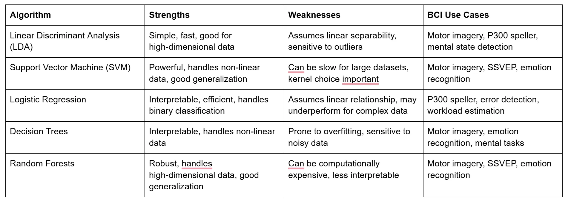
The best classification algorithm for your BCI application depends on several factors, including the nature of your data, the complexity of the task, and the desired balance between accuracy, speed, and interpretability. Here's a table comparing some common algorithms:
Cross-Validation and Performance Metrics: Evaluating Your BCI Model
We've trained our BCI model to decode brain signals, but how do we know if it's any good? Simply evaluating its performance on the same data it was trained on can be misleading. This is where cross-validation and performance metrics come to the rescue, providing robust tools to assess our model's true capabilities and ensure it generalizes well to unseen EEG data.
Why Cross-Validation? Ensuring Your BCI Doesn't Just Memorize
Imagine training a BCI model to detect fatigue based on EEG signals. If we only evaluate its performance on the same data it was trained on, it might simply memorize the patterns in that specific dataset, achieving high accuracy but failing to generalize to new EEG recordings from different individuals or under varying conditions. This is called overfitting.
Cross-validation is a technique for evaluating a machine learning model by training it on multiple subsets of the data and testing it on the remaining data. This helps us assess how well the model generalizes to unseen data, providing a more realistic estimate of its performance in real-world BCI applications.
K-Fold Cross-Validation: A Robust Evaluation Strategy
K-fold cross-validation is a popular cross-validation method that involves dividing the data into k equal-sized folds. The model is trained on k-1 folds and tested on the remaining fold. This process is repeated k times, with each fold serving as the test set once. The performance scores from each iteration are then averaged to obtain a robust estimate of the model's performance.
Scikit-learn makes implementing k-fold cross-validation straightforward:
from sklearn.model_selection import cross_val_score
# Perform 5-fold cross-validation on an SVM classifier
scores = cross_val_score(svm, X, y, cv=5)
# Print the average accuracy across the folds
print("Average accuracy: %0.2f" % scores.mean())
This code performs 5-fold cross-validation using an SVM classifier and prints the average accuracy across the folds.
Performance Metrics: Measuring BCI Success
Evaluating a BCI model involves more than just looking at overall accuracy. Different performance metrics provide insights into specific aspects of the model's behavior, helping us understand its strengths and weaknesses.
Here are some essential metrics for BCI classification:
- Accuracy: The proportion of correctly classified instances. While accuracy is a useful overall measure, it can be misleading if the classes are imbalanced (e.g., many more examples of one mental state than another).
- Precision: The proportion of correctly classified positive instances out of all instances classified as positive. High precision indicates a low rate of false positives, important for BCIs where incorrect actions could have consequences (e.g., controlling a wheelchair).
- Recall (Sensitivity): The proportion of correctly classified positive instances out of all actual positive instances. High recall indicates a low rate of false negatives, crucial for BCIs where missing a user's intention is critical (e.g., detecting emergency signals).
- F1-Score: The harmonic mean of precision and recall, providing a balanced measure that considers both false positives and false negatives.
- Confusion Matrix: A visualization that shows the counts of true positives, true negatives, false positives, and false negatives, providing a detailed overview of the model's classification performance.
Scikit-learn offers functions for calculating these metrics:
from sklearn.metrics import accuracy_score, precision_score, recall_score, f1_score, confusion_matrix
# Calculate accuracy
accuracy = accuracy_score(y_test, y_pred)
# Calculate precision
precision = precision_score(y_test, y_pred)
# Calculate recall
recall = recall_score(y_test, y_pred)
# Calculate F1-score
f1 = f1_score(y_test, y_pred)
# Create a confusion matrix
cm = confusion_matrix(y_test, y_pred)
Hyperparameter Tuning: Fine-Tuning Your BCI for Peak Performance
Most machine learning algorithms have hyperparameters, settings that control the learning process and influence the model's performance. For example, the C parameter in an SVM controls the trade-off between maximizing the margin and minimizing classification errors.
Hyperparameter tuning involves finding the optimal values for these hyperparameters to achieve the best performance on our specific dataset and BCI application. Techniques like grid search and randomized search systematically explore different hyperparameter combinations, guided by cross-validation performance, to find the settings that yield the best results.
Introduction to Deep Learning for BCI: Exploring the Frontier
We've explored powerful machine learning techniques for BCI, but the field is constantly evolving. Deep learning, a subfield of machine learning inspired by the structure and function of the human brain, is pushing the boundaries of BCI capabilities, enabling more sophisticated decoding of brain signals and opening up new possibilities for human-computer interaction.
What is Deep Learning? Unlocking Complex Patterns with Artificial Neural Networks
Deep learning algorithms, particularly artificial neural networks (ANNs), are designed to learn complex patterns and representations from data. ANNs consist of interconnected layers of artificial neurons, mimicking the interconnected structure of the brain.
Through a process called training, ANNs learn to adjust the connections between neurons, enabling them to extract increasingly abstract and complex features from the data. This hierarchical feature learning allows deep learning models to capture intricate patterns in EEG data that traditional machine learning algorithms might miss.
Deep Learning for BCI: Architectures for Decoding Brainwaves
Several deep learning architectures have proven particularly effective for EEG analysis:
- Convolutional Neural Networks (CNNs): Excel at capturing spatial patterns in data, making them suitable for analyzing multi-channel EEG recordings. CNNs are often used for motor imagery BCIs, where they can learn to recognize patterns of brain activity associated with different imagined movements.
- Recurrent Neural Networks (RNNs): Designed to handle sequential data, making them well-suited for analyzing the temporal dynamics of EEG signals. RNNs are used in applications like emotion recognition from EEG, where they can learn to identify patterns of brain activity that unfold over time.
Benefits and Challenges: Weighing the Potential of Deep Learning
Deep learning offers several potential benefits for BCI:
- Higher Accuracy: Deep learning models can achieve higher accuracy than traditional machine learning algorithms, particularly for complex BCI tasks.
- Automatic Feature Learning: Deep learning models can automatically learn relevant features from raw data, reducing the need for manual feature engineering.
However, deep learning also presents challenges:
- Larger Datasets: Deep learning models typically require larger datasets for training than traditional machine learning algorithms.
- Computational Resources: Training deep learning models can be computationally demanding, requiring specialized hardware like GPUs.
Empowering BCIs with Intelligent Algorithms
From feature selection to classification algorithms and the frontier of deep learning, we've explored a powerful toolkit for decoding brain signals using machine learning. These techniques are transforming the field of BCIs, enabling the development of more accurate, reliable, and sophisticated systems that can translate brain activity into action.
Resources and Further Reading
- Tutorial: Scikit-learn documentation: https://scikit-learn.org/stable/
- Article: Lotte, F., Bougrain, L., Cichocki, A., Clerc, M., Congedo, M., Rakotomamonjy, A., & Yger, F. (2018). A review of classification algorithms for EEG-based brain–computer interfaces: a 10-year update. Journal of Neural Engineering, 15(3), 031005.
Time to Build: Creating a P300 Speller with Python
This concludes our exploration of essential machine learning techniques for BCI. You've gained a solid understanding of how to select relevant features, train classification models, evaluate their performance, and even glimpse the potential of deep learning.
In the next post, we'll put these techniques into practice by building our own P300 speller, a classic BCI application that allows users to communicate by focusing their attention on letters on a screen. Get ready for a hands-on adventure in BCI development!
BCI Kickstarter #07 : Building a P300 Speller: Translating Brainwaves into Letters
Welcome back to our BCI crash course! We've explored the foundations of BCIs, delved into the intricacies of brain signals, mastered the art of signal processing, and learned how to train intelligent algorithms to decode those signals. Now, we are ready to put all this knowledge into action by building a real-world BCI application: a P300 speller. P300 spellers are a groundbreaking technology that allows individuals with severe motor impairments to communicate by simply focusing their attention on letters on a screen. By harnessing the power of the P300 event-related potential, a brain response elicited by rare or surprising stimuli, these spellers open up a world of communication possibilities for those who might otherwise struggle to express themselves. In this blog, we will guide you through the step-by-step process of building a P300 speller using Python, MNE-Python, and scikit-learn. Get ready for a hands-on adventure in BCI development as we translate brainwaves into letters and words!
Step-by-Step Implementation: A Hands-on BCI Project
1. Loading the Dataset
Introducing the BNCI Horizon 2020 Dataset: A Rich Resource for P300 Speller Development
For this project, we'll use the BNCI Horizon 2020 dataset, a publicly available EEG dataset specifically designed for P300 speller research. This dataset offers several advantages:
- Large Sample Size: It includes recordings from a substantial number of participants, providing a diverse range of P300 responses.
- Standardized Paradigm: The dataset follows a standardized experimental protocol, ensuring consistency and comparability across recordings.
- Detailed Metadata: It provides comprehensive metadata, including information about stimulus presentation, participant responses, and electrode locations.
This dataset is well-suited for our P300 speller project because it provides high-quality EEG data recorded during a classic P300 speller paradigm, allowing us to focus on the core signal processing and machine learning steps involved in building a functional speller.
Loading the Data with MNE-Python: Accessing the Brainwave Symphony
To load the BNCI Horizon 2020 dataset using MNE-Python, you'll need to download the data files from the dataset's website (http://bnci-horizon-2020.eu/database/data-sets). Once you have the files, you can use the following code snippet to load a specific participant's data:
import mne
# Set the path to the dataset directory
data_path = '<path_to_dataset_directory>'
# Load the raw EEG data for a specific participant
raw = mne.io.read_raw_gdf(data_path + '/A01T.gdf', preload=True)
Replace <path_to_dataset_directory> with the actual path to the directory where you've stored the dataset files. This code loads the EEG data for participant "A01" during the training session ("T").
2. Data Preprocessing: Refining the EEG Signals for P300 Detection
Raw EEG data is often a mixture of brain signals, artifacts, and noise. Before we can effectively detect the P300 component, we need to clean up the data and isolate the relevant frequencies.
Channel Selection: Focusing on the P300's Neighborhood
The P300 component is typically most prominent over the central-parietal region of the scalp. Therefore, we'll select channels that capture activity from this area. Commonly used channels for P300 detection include:
- Cz: The electrode located at the vertex of the head, directly over the central sulcus.
- Pz: The electrode located over the parietal lobe, slightly posterior to Cz.
- Surrounding Electrodes: Additional electrodes surrounding Cz and Pz, such as CPz, FCz, and P3/P4, can also provide valuable information.
These electrodes are chosen because they tend to be most sensitive to the positive voltage deflection that characterizes the P300 response.
# Select the desired channels
channels = ['Cz', 'Pz', 'CPz', 'FCz', 'P3', 'P4']
# Create a new raw object with only the selected channels
raw_selected = raw.pick_channels(channels)
Filtering: Tuning into the P300 Frequency
The P300 component is a relatively slow brainwave, typically occurring in the frequency range of 0.1 Hz to 10 Hz. Filtering helps us remove unwanted frequencies outside this range, enhancing the signal-to-noise ratio for P300 detection.
We'll apply a band-pass filter to the selected EEG channels, using cutoff frequencies of 0.1 Hz and 10 Hz:
# Apply a band-pass filter from 0.1 Hz to 10 Hz
raw_filtered = raw_selected.filter(l_freq=0.1, h_freq=10)
This filter removes slow drifts (below 0.1 Hz) and high-frequency noise (above 10 Hz), allowing the P300 component to stand out more clearly.
Artifact Removal (Optional): Combating Unwanted Signals
Depending on the quality of the EEG data and the presence of artifacts, we might need to apply additional artifact removal techniques. Independent Component Analysis (ICA) is a powerful method for separating independent sources of activity in EEG recordings. If the BNCI Horizon 2020 dataset contains significant artifacts, we can use ICA to identify and remove components related to eye blinks, muscle activity, or other sources of interference.
3. Epoching and Averaging: Isolating the P300 Response
To capture the brain's response to specific stimuli, we'll create epochs, time-locked segments of EEG data centered around events of interest.
Defining Epochs: Capturing the P300 Time Window
We'll define epochs around both target stimuli (the letters the user is focusing on) and non-target stimuli (all other letters). The epoch time window should capture the P300 response, typically occurring between 300 and 500 milliseconds after the stimulus onset. We'll use a window of -200 ms to 800 ms to include a baseline period and capture the full P300 waveform.
# Define event IDs for target and non-target stimuli (refer to dataset documentation)
event_id = {'target': 1, 'non-target': 0}
# Set the epoch time window
tmin = -0.2 # 200 ms before stimulus onset
tmax = 0.8 # 800 ms after stimulus onset
# Create epochs
epochs = mne.Epochs(raw_filtered, events, event_id, tmin, tmax, baseline=(-0.2, 0), preload=True)
Baseline Correction: Removing Pre-Stimulus Bias
Baseline correction involves subtracting the average activity during the baseline period (-200 ms to 0 ms) from each epoch. This removes any pre-existing bias in the EEG signal, ensuring that the measured response is truly due to the stimulus.
Averaging Evoked Responses: Enhancing the P300 Signal
To enhance the P300 signal and reduce random noise, we'll average the epochs for target and non-target stimuli separately. This averaging process reveals the event-related potential (ERP), a characteristic waveform reflecting the brain's response to the stimulus.
# Average the epochs for target and non-target stimuli
evoked_target = epochs['target'].average()
evoked_non_target = epochs['non-target'].average()
4. Feature Extraction: Quantifying the P300
Selecting Features: Capturing the P300's Signature
The P300 component is characterized by a positive voltage deflection peaking around 300-500 ms after the stimulus onset. We'll select features that capture this signature:
- Peak Amplitude: The maximum amplitude of the P300 component.
- Mean Amplitude: The average amplitude within a specific time window around the P300 peak.
- Latency: The time it takes for the P300 component to reach its peak amplitude.
These features provide a quantitative representation of the P300 response, allowing us to train a classifier to distinguish between target and non-target stimuli.
Extracting Features: From Waveforms to Numbers
We can extract these features from the averaged evoked responses using MNE-Python's functions:
# Extract peak amplitude
peak_amplitude_target = evoked_target.get_data().max(axis=1)
peak_amplitude_non_target = evoked_non_target.get_data().max(axis=1)
# Extract mean amplitude within a time window (e.g., 300 ms to 500 ms)
mean_amplitude_target = evoked_target.crop(tmin=0.3, tmax=0.5).get_data().mean(axis=1)
mean_amplitude_non_target = evoked_non_target.crop(tmin=0.3, tmax=0.5).get_data().mean(axis=1)
# Extract latency of the P300 peak
latency_target = evoked_target.get_peak(tmin=0.3, tmax=0.5)[1]
latency_non_target = evoked_non_target.get_peak(tmin=0.3, tmax=0.5)[1]
5. Classification: Training the Brainwave Decoder
Choosing a Classifier: LDA for P300 Speller Decoding
Linear Discriminant Analysis (LDA) is a suitable classifier for P300 spellers due to its simplicity, efficiency, and ability to handle high-dimensional data. It seeks to find a linear combination of features that best separates the classes (target vs. non-target).
Training the Model: Learning from Brainwaves
We'll train the LDA classifier using the extracted features:
from sklearn.discriminant_analysis import LinearDiscriminantAnalysis
# Create an LDA object
lda = LinearDiscriminantAnalysis()
# Combine the features into a data matrix
X = np.vstack((peak_amplitude_target, peak_amplitude_non_target,
mean_amplitude_target, mean_amplitude_non_target,
latency_target, latency_non_target)).T
# Create a label vector (1 for target, 0 for non-target)
y = np.concatenate((np.ones(len(peak_amplitude_target)), np.zeros(len(peak_amplitude_non_target))))
# Train the LDA model
lda.fit(X, y)
Feature selection plays a crucial role here. By choosing features that effectively capture the P300 response, we improve the classifier's ability to distinguish between target and non-target stimuli.
6. Visualization: Validating Our Progress
Visualizing Preprocessed Data and P300 Responses
Visualizations help us understand the data and validate our preprocessing steps:
- Plot Averaged Epochs: Use evoked_target.plot() and evoked_non_target.plot() to visualize the average target and non-target epochs, confirming the presence of the P300 component in the target epochs.
- Topographical Plot: Use evoked_target.plot_topomap() to visualize the scalp distribution of the P300 component, ensuring it's most prominent over the expected central-parietal region.
Performance Evaluation: Assessing Speller Accuracy
Now that we've built our P300 speller, it's crucial to evaluate its performance. We need to assess how accurately it can distinguish between target and non-target stimuli, and consider practical factors that might influence its usability in real-world settings.
Cross-Validation: Ensuring Robustness and Generalizability
To obtain a reliable estimate of our speller's performance, we'll use k-fold cross-validation. This technique involves splitting the data into k folds, training the model on k-1 folds, and testing it on the remaining fold. Repeating this process k times, with each fold serving as the test set once, gives us a robust measure of the model's ability to generalize to unseen data.
from sklearn.model_selection import cross_val_score
# Perform 5-fold cross-validation
scores = cross_val_score(lda, X, y, cv=5)
# Print the average accuracy across the folds
print("Average accuracy: %0.2f" % scores.mean())
This code performs 5-fold cross-validation using our trained LDA classifier and prints the average accuracy across the folds.
Metrics for P300 Spellers: Beyond Accuracy
While accuracy is a key metric for P300 spellers, indicating the proportion of correctly classified stimuli, other metrics provide additional insights:
- Information Transfer Rate (ITR): Measures the speed of communication, taking into account the number of possible choices and the accuracy of selection. A higher ITR indicates a faster and more efficient speller.
Practical Considerations: Bridging the Gap to Real-World Use
Several practical factors can influence the performance and usability of P300 spellers:
- User Variability: P300 responses can vary significantly between individuals due to factors like age, attention, and neurological conditions. To address this, personalized calibration is crucial, where the speller is adjusted to each user's unique brain responses. Adaptive algorithms can also be employed to continuously adjust the speller based on the user's performance.
- Fatigue and Attention: Prolonged use can lead to fatigue and decreased attention, affecting P300 responses and speller accuracy. Strategies to mitigate this include incorporating breaks, using engaging stimuli, and employing algorithms that can detect and adapt to changes in user state.
- Training Duration: The amount of training a user receives can impact their proficiency with the speller. Sufficient training is essential for users to learn to control their P300 responses and achieve optimal performance.
Empowering Communication with P300 Spellers
We've successfully built a P300 speller, witnessing firsthand the power of EEG, signal processing, and machine learning to create a functional BCI application. These spellers hold immense potential as a communication tool, enabling individuals with severe motor impairments to express themselves, connect with others, and participate more fully in the world.
Further Reading and Resources
- Review article: Pan J et al. Advances in P300 brain-computer interface spellers: toward paradigm design and performance evaluation. Front Hum Neurosci. 2022 Dec 21;16:1077717. doi: 10.3389/fnhum.2022.1077717. PMID: 36618996; PMCID: PMC9810759.
- Dataset: BNCI Horizon 2020 P300 dataset: http://bnci-horizon-2020.eu/database/data-sets
- Tutorial: PyQt documentation for GUI development (optional): https://doc.qt.io/qtforpython/
Future Directions: Advancing P300 Speller Technology
The field of P300 speller development is constantly evolving. Emerging trends include:
- Deep Learning: Applying deep learning algorithms to improve P300 detection accuracy and robustness.
- Multimodal BCIs: Combining EEG with other brain imaging modalities (e.g., fNIRS) or physiological signals (e.g., eye tracking) to enhance speller performance.
- Hybrid Approaches: Integrating P300 spellers with other BCI paradigms (e.g., motor imagery) to create more flexible and versatile communication systems.
Next Stop: Motor Imagery BCIs
In the next blog post, we'll explore motor imagery BCIs, a fascinating paradigm where users control devices by simply imagining movements. We'll dive into the brain signals associated with motor imagery, learn how to extract features, and build a classifier to decode these intentions.
BCI Kickstarter #08 : Developing a Motor Imagery BCI: Controlling Devices with Your Mind
Welcome back to our BCI crash course! We've journeyed from the fundamental concepts of BCIs to the intricacies of brain signals, mastered the art of signal processing, and learned how to train intelligent algorithms to decode those signals. Now, we're ready to tackle a fascinating and powerful BCI paradigm: motor imagery. Motor imagery BCIs allow users to control devices simply by imagining movements. This technology holds immense potential for applications like controlling neuroprosthetics for individuals with paralysis, assisting in stroke rehabilitation, and even creating immersive gaming experiences. In this post, we'll guide you through the step-by-step process of building a basic motor imagery BCI using Python, MNE-Python, and scikit-learn. Get ready to harness the power of your thoughts to interact with technology!
Understanding Motor Imagery: The Brain's Internal Rehearsal
Before we dive into building our BCI, let's first understand the fascinating phenomenon of motor imagery.
What is Motor Imagery? Moving Without Moving
Motor imagery is the mental rehearsal of a movement without actually performing the physical action. It's like playing a video of the movement in your mind's eye, engaging the same neural processes involved in actual execution but without sending the final commands to your muscles.
Neural Basis of Motor Imagery: The Brain's Shared Representations
Remarkably, motor imagery activates similar brain regions and neural networks as actual movement. The motor cortex, the area of the brain responsible for planning and executing movements, is particularly active during motor imagery. This shared neural representation suggests that imagining a movement is a powerful way to engage the brain's motor system, even without physical action.
EEG Correlates of Motor Imagery: Decoding Imagined Movements
Motor imagery produces characteristic changes in EEG signals, particularly over the motor cortex. Two key features are:
- Event-Related Desynchronization (ERD): A decrease in power in specific frequency bands (mu, 8-12 Hz, and beta, 13-30 Hz) over the motor cortex during motor imagery. This decrease reflects the activation of neural populations involved in planning and executing the imagined movement.
- Event-Related Synchronization (ERS): An increase in power in those frequency bands after the termination of motor imagery, as the brain returns to its resting state.
These EEG features provide the foundation for decoding motor imagery and building BCIs that can translate imagined movements into control signals.
Building a Motor Imagery BCI: A Step-by-Step Guide
Now that we understand the neural basis of motor imagery, let's roll up our sleeves and build a BCI that can decode these imagined movements. We'll follow a step-by-step process, using Python, MNE-Python, and scikit-learn to guide us.
1. Loading the Dataset
Choosing the Dataset: BCI Competition IV Dataset 2a
For this project, we'll use the BCI Competition IV dataset 2a, a publicly available EEG dataset specifically designed for motor imagery BCI research. This dataset offers several advantages:
- Standardized Paradigm: The dataset follows a well-defined experimental protocol, making it easy to understand and replicate. Participants were instructed to imagine moving their left or right hand, providing clear labels for our classification task.
- Multiple Subjects: It includes recordings from nine subjects, providing a decent sample size to train and evaluate our BCI model.
- Widely Used: This dataset has been extensively used in BCI research, allowing us to compare our results with established benchmarks and explore various analysis approaches.
You can download the dataset from the BCI Competition IV website (http://www.bbci.de/competition/iv/).
Loading the Data: MNE-Python to the Rescue
Once you have the dataset downloaded, you can load it using MNE-Python's convenient functions. Here's a code snippet to get you started:
import mne
# Set the path to the dataset directory
data_path = '<path_to_dataset_directory>'
# Load the raw EEG data for subject 1
raw = mne.io.read_raw_gdf(data_path + '/A01T.gdf', preload=True)
Replace <path_to_dataset_directory> with the actual path to the directory where you've stored the dataset files. This code loads the data for subject "A01" from the training session ("T").
2. Data Preprocessing: Preparing the Signals for Decoding
Raw EEG data is often noisy and contains artifacts that can interfere with our analysis. Preprocessing is crucial for cleaning up the data and isolating the relevant brain signals associated with motor imagery.
Channel Selection: Focusing on the Motor Cortex
Since motor imagery primarily activates the motor cortex, we'll select EEG channels that capture activity from this region. Key channels include:
- C3: Located over the left motor cortex, sensitive to right-hand motor imagery.
- C4: Located over the right motor cortex, sensitive to left-hand motor imagery.
- Cz: Located over the midline, often used as a reference or to capture general motor activity.
# Select the desired channels
channels = ['C3', 'C4', 'Cz']
# Create a new raw object with only the selected channels
raw_selected = raw.pick_channels(channels)
Filtering: Isolating Mu and Beta Rhythms
We'll apply a band-pass filter to isolate the mu (8-12 Hz) and beta (13-30 Hz) frequency bands, as these rhythms exhibit the most prominent ERD/ERS patterns during motor imagery.
# Apply a band-pass filter from 8 Hz to 30 Hz
raw_filtered = raw_selected.filter(l_freq=8, h_freq=30)
This filtering step removes irrelevant frequencies and enhances the signal-to-noise ratio for detecting motor imagery-related brain activity.
Artifact Removal: Enhancing Data Quality (Optional)
Depending on the dataset and the quality of the recordings, we might need to apply artifact removal techniques. Independent Component Analysis (ICA) is particularly useful for identifying and removing artifacts like eye blinks, muscle activity, and heartbeats, which can contaminate our motor imagery signals. MNE-Python provides functions for performing ICA and visualizing the components, allowing us to select and remove those associated with artifacts. This step can significantly improve the accuracy and reliability of our motor imagery BCI.
3. Epoching and Visualizing: Zooming in on Motor Imagery
Now that we've preprocessed our EEG data, let's create epochs around the motor imagery cues, allowing us to focus on the brain activity specifically related to those imagined movements.
Defining Epochs: Capturing the Mental Rehearsal
The BCI Competition IV dataset 2a includes event markers indicating the onset of the motor imagery cues. We'll use these markers to create epochs, typically spanning a time window from a second before the cue to several seconds after it. This window captures the ERD and ERS patterns associated with motor imagery.
# Define event IDs for left and right hand motor imagery (refer to dataset documentation)
event_id = {'left_hand': 1, 'right_hand': 2}
# Set the epoch time window
tmin = -1 # 1 second before the cue
tmax = 4 # 4 seconds after the cue
# Create epochs
epochs = mne.Epochs(raw_filtered, events, event_id, tmin, tmax, baseline=(-1, 0), preload=True)
Baseline Correction: Removing Pre-Imagery Bias
We'll apply baseline correction to remove any pre-existing bias in the EEG signal, ensuring that our analysis focuses on the changes specifically related to motor imagery.
Visualizing: Inspecting and Gaining Insights
- Plotting Epochs: Use epochs.plot() to visualize individual epochs, inspecting for artifacts and observing the general patterns of brain activity during motor imagery.
- Topographical Maps: Use epochs['left_hand'].average().plot_topomap() and epochs['right_hand'].average().plot_topomap() to visualize the scalp distribution of mu and beta power changes during left and right hand motor imagery. These maps can help validate our channel selection and confirm that the ERD patterns are localized over the expected motor cortex areas.
4. Feature Extraction with Common Spatial Patterns (CSP): Maximizing Class Differences
Common Spatial Patterns (CSP) is a spatial filtering technique specifically designed to extract features that best discriminate between two classes of EEG data. In our case, these classes are left-hand and right-hand motor imagery.
Understanding CSP: Finding Optimal Spatial Filters
CSP seeks to find spatial filters that maximize the variance of one class while minimizing the variance of the other. It achieves this by solving an eigenvalue problem based on the covariance matrices of the two classes. The resulting spatial filters project the EEG data onto a new space where the classes are more easily separable
.
Applying CSP: MNE-Python's CSP Function
MNE-Python's mne.decoding.CSP() function makes it easy to extract CSP features:
from mne.decoding import CSP
# Create a CSP object
csp = CSP(n_components=4, reg=None, log=True, norm_trace=False)
# Fit the CSP to the epochs data
csp.fit(epochs['left_hand'].get_data(), epochs['right_hand'].get_data())
# Transform the epochs data using the CSP filters
X_csp = csp.transform(epochs.get_data())
Interpreting CSP Filters: Mapping Brain Activity
The CSP spatial filters represent patterns of brain activity that differentiate between left and right hand motor imagery. By visualizing these filters, we can gain insights into the underlying neural sources involved in these imagined movements.
Selecting CSP Components: Balancing Performance and Complexity
The n_components parameter in the CSP() function determines the number of CSP components to extract. Choosing the optimal number of components is crucial for balancing classification performance and model complexity. Too few components might not capture enough information, while too many can lead to overfitting. Cross-validation can help us find the optimal balance.
5. Classification with a Linear SVM: Decoding Motor Imagery
Choosing the Classifier: Linear SVM for Simplicity and Efficiency
We'll use a linear Support Vector Machine (SVM) to classify our motor imagery data. Linear SVMs are well-suited for this task due to their simplicity, efficiency, and ability to handle high-dimensional data. They seek to find a hyperplane that best separates the two classes in the feature space.
Training the Model: Learning from Spatial Patterns
from sklearn.svm import SVC
# Create a linear SVM classifier
svm = SVC(kernel='linear')
# Train the SVM model
svm.fit(X_csp_train, y_train)
Hyperparameter Tuning: Optimizing for Peak Performance
SVMs have hyperparameters, like the regularization parameter C, that control the model's complexity and generalization ability. Hyperparameter tuning, using techniques like grid search or cross-validation, helps us find the optimal values for these parameters to maximize classification accuracy.
Evaluating the Motor Imagery BCI: Measuring Mind Control
We've built our motor imagery BCI, but how well does it actually work? Evaluating its performance is crucial for understanding its capabilities and limitations, especially if we envision real-world applications.
Cross-Validation: Assessing Generalizability
To obtain a reliable estimate of our BCI's performance, we'll employ k-fold cross-validation. This technique helps us assess how well our model generalizes to unseen data, providing a more realistic measure of its real-world performance.
from sklearn.model_selection import cross_val_score
# Perform 5-fold cross-validation
scores = cross_val_score(svm, X_csp, y, cv=5)
# Print the average accuracy across the folds
print("Average accuracy: %0.2f" % scores.mean())
Performance Metrics: Beyond Simple Accuracy
- Accuracy: While accuracy, the proportion of correctly classified instances, is a useful starting point, it doesn't tell the whole story. For imbalanced datasets (where one class has significantly more samples than the other), accuracy can be misleading.
- Kappa Coefficient: The Kappa coefficient (κ) measures the agreement between the classifier's predictions and the true labels, taking into account the possibility of chance agreement. A Kappa value of 1 indicates perfect agreement, while 0 indicates agreement equivalent to chance. Kappa is a more robust metric than accuracy, especially for imbalanced datasets.
- Information Transfer Rate (ITR): ITR quantifies the amount of information transmitted by the BCI per unit of time, considering both accuracy and the number of possible choices. A higher ITR indicates a faster and more efficient communication system.
- Sensitivity and Specificity: These metrics provide a more nuanced view of classification performance. Sensitivity measures the proportion of correctly classified positive instances (e.g., correctly identifying left-hand imagery), while specificity measures the proportion of correctly classified negative instances (e.g., correctly identifying right-hand imagery).
Practical Implications: From Benchmarks to Real-World Use
Evaluating a motor imagery BCI goes beyond just looking at numbers. We need to consider the practical implications of its performance:
- Minimum Accuracy Requirements: Real-world applications often have minimum accuracy thresholds. For example, a neuroprosthetic controlled by a motor imagery BCI might require an accuracy of over 90% to ensure safe and reliable operation.
- User Experience: Beyond accuracy, factors like speed, ease of use, and mental effort also contribute to the overall user experience.
Unlocking the Potential of Motor Imagery BCIs
We've successfully built a basic motor imagery BCI, witnessing the power of EEG, signal processing, and machine learning to decode movement intentions directly from brain signals. Motor imagery BCIs hold immense potential for a wide range of applications, offering new possibilities for individuals with disabilities, stroke rehabilitation, and even immersive gaming experiences.
Resources for Further Reading
- Review article: EEG-Based Brain-Computer Interfaces Using Motor-Imagery: Techniques and Challenges https://www.ncbi.nlm.nih.gov/pmc/articles/PMC6471241/
- Review article: A review of critical challenges in MI-BCI: From conventional to deep learning methods https://www.sciencedirect.com/science/article/abs/pii/S016502702200262X
- BCI Competition IV Dataset 2a https://www.bbci.de/competition/iv/desc_2a.pdf
From Motor Imagery to Advanced BCI Paradigms
This concludes our exploration of building a motor imagery BCI. You've gained valuable insights into the neural basis of motor imagery, learned how to extract features using CSP, trained a classifier to decode movement intentions, and evaluated the performance of your BCI model.
In our final blog post, we'll explore the exciting frontier of advanced BCI paradigms and future directions. We'll delve into concepts like hybrid BCIs, adaptive algorithms, ethical considerations, and the ever-expanding possibilities that lie ahead in the world of brain-computer interfaces. Stay tuned for a glimpse into the future of mind-controlled technology!
BCI Kickstarter #09 : Advanced Topics and Future Directions in BCI: Pushing the Boundaries of Mind-Controlled Technology
Welcome back to our BCI crash course! Over the past eight blogs, we have explored the fascinating intersection of neuroscience, engineering, and machine learning, from the fundamental concepts of BCIs to the practical implementation of real-world applications. In this final installment, we will shift our focus to the future of BCI, delving into advanced topics and research directions that are pushing the boundaries of mind-controlled technology. Get ready to explore the exciting possibilities of hybrid BCIs, adaptive algorithms, ethical considerations, and the transformative potential that lies ahead for this groundbreaking field.
Hybrid BCIs: Combining Paradigms for Enhanced Performance
As we've explored in previous posts, different BCI paradigms leverage distinct brain signals and have their strengths and limitations. Motor imagery BCIs excel at decoding movement intentions, P300 spellers enable communication through attention-based selections, and SSVEP BCIs offer high-speed control using visual stimuli.
What are Hybrid BCIs? Synergy of Brain Signals
Hybrid BCIs combine multiple BCI paradigms, integrating different brain signals to create more robust, versatile, and user-friendly systems. Imagine a BCI that leverages both motor imagery and SSVEP to control a robotic arm with greater precision and flexibility, or a system that combines P300 with error-related potentials (ErrPs) to improve the accuracy and speed of a speller.
Benefits of Hybrid BCIs: Unlocking New Possibilities
Hybrid BCIs offer several advantages over single-paradigm systems:
- Improved Accuracy and Reliability: Combining complementary brain signals can enhance the signal-to-noise ratio and reduce the impact of individual variations in brain activity, leading to more accurate and reliable BCI control.
- Increased Flexibility and Adaptability: Hybrid BCIs can adapt to different user needs, tasks, and environments by dynamically switching between paradigms or combining them in a way that optimizes performance.
- Richer and More Natural Interactions: Integrating multiple BCI paradigms opens up possibilities for creating more intuitive and natural BCI interactions, allowing users to control devices with a greater range of mental commands.
Examples of Hybrid BCIs: Innovations in Action
Research is exploring various hybrid BCI approaches:
- Motor Imagery + SSVEP: Combining motor imagery with SSVEP can enhance the control of robotic arms. Motor imagery provides continuous control signals for movement direction, while SSVEP enables discrete selections for grasping or releasing objects.
- P300 + ErrP: Integrating P300 with ErrPs, brain signals that occur when we make errors, can improve speller accuracy. The P300 is used to select letters, while ErrPs can be used to automatically correct errors, reducing the need for manual backspacing.
Adaptive BCIs: Learning and Evolving with the User
One of the biggest challenges in BCI development is the inherent variability in brain signals. A BCI system that works perfectly for one user might perform poorly for another, and even a single user's brain activity can change over time due to factors like learning, fatigue, or changes in attention. This is where adaptive BCIs come into play, offering a dynamic and personalized approach to brain-computer interaction.
The Need for Adaptation: Embracing the Brain's Dynamic Nature
BCI systems need to adapt to several factors:
- Changes in User Brain Activity: Brain signals are not static. They evolve as users learn to control the BCI, become fatigued, or shift their attention. An adaptive BCI can track these changes and adjust its processing accordingly.
- Variations in Signal Quality and Noise: EEG recordings can be affected by various sources of noise, from muscle artifacts to environmental interference. An adaptive BCI can adjust its filtering and artifact rejection parameters to maintain optimal signal quality.
- Different User Preferences and Skill Levels: BCI users have different preferences for control strategies, feedback modalities, and interaction speeds. An adaptive BCI can personalize its settings to match each user's individual needs and skill level.
Methods for Adaptation: Tailoring BCIs to the Individual
Various techniques can be employed to create adaptive BCIs:
- Machine Learning Adaptation: Machine learning algorithms, such as those used for classification, can be trained to continuously learn and update the BCI model based on the user's brain data. This allows the BCI to adapt to changes in brain patterns over time and improve its accuracy and responsiveness.
- User Feedback Adaptation: BCIs can incorporate user feedback, either explicitly (through direct input) or implicitly (by monitoring performance and user behavior), to adjust parameters and optimize the interaction. For example, if a user consistently struggles to control a motor imagery BCI, the system could adjust the classification thresholds or provide more frequent feedback to assist them.
Benefits of Adaptive BCIs: A Personalized and Evolving Experience
Adaptive BCIs offer significant advantages:
- Enhanced Usability and User Experience: By adapting to individual needs and preferences, adaptive BCIs can become more intuitive and easier to use, reducing user frustration and improving the overall experience.
- Improved Long-Term Performance and Reliability: Adaptive BCIs can maintain high levels of performance and reliability over time by adjusting to changes in brain activity and signal quality.
- Personalized BCIs: Adaptive algorithms can tailor the BCI to each user's unique brain patterns, preferences, and abilities, creating a truly personalized experience.
Ethical Considerations: Navigating the Responsible Development of BCI
As BCI technology advances, it's crucial to consider the ethical implications of its development and use. BCIs have the potential to profoundly impact individuals and society, raising questions about privacy, autonomy, fairness, and responsibility.
Introduction: Ethics at the Forefront of BCI Innovation
Ethical considerations should be woven into the fabric of BCI research and development, guiding our decisions and ensuring that this powerful technology is used for good.
Key Ethical Concerns: Navigating a Complex Landscape
- Privacy and Data Security: BCIs collect sensitive brain data, raising concerns about privacy violations and potential misuse. Robust data security measures and clear ethical guidelines are crucial for protecting user privacy and ensuring responsible data handling.
- Agency and Autonomy: BCIs have the potential to influence user thoughts, emotions, and actions. It's essential to ensure that BCI use respects user autonomy and agency, avoiding coercion, manipulation, or unintended consequences.
- Bias and Fairness: BCI algorithms can inherit biases from the data they are trained on, potentially leading to unfair or discriminatory outcomes. Addressing these biases and developing fair and equitable BCI systems is essential for responsible innovation.
- Safety and Responsibility: As BCIs become more sophisticated and integrated into critical applications like healthcare and transportation, ensuring their safety and reliability is paramount. Clear lines of responsibility and accountability need to be established to mitigate potential risks and ensure ethical use.
Guidelines and Principles: A Framework for Responsible BCI
Efforts are underway to establish ethical guidelines and principles for BCI research and development. These guidelines aim to promote responsible innovation, protect user rights, and ensure that BCI technology benefits society as a whole.
Current Challenges and Future Prospects: The Road Ahead for BCI
While BCI technology has made remarkable progress, several challenges remain to be addressed before it can fully realize its transformative potential. However, the future of BCI is bright, with exciting possibilities on the horizon for enhancing human capabilities, restoring lost function, and improving lives.
Technical Challenges: Overcoming Roadblocks to Progress
- Signal Quality and Noise: Non-invasive BCIs, particularly those based on EEG, often suffer from low signal-to-noise ratios. Improving signal quality through advanced electrode designs, noise reduction algorithms, and a better understanding of brain signals is crucial for enhancing BCI accuracy and reliability.
- Robustness and Generalizability: Current BCI systems often work well in controlled laboratory settings but struggle to perform consistently across different users, environments, and tasks. Developing more robust and generalizable BCIs is essential for wider adoption and real-world applications.
- Long-Term Stability: Maintaining the long-term stability and performance of BCI systems, especially for implanted devices, is a significant challenge. Addressing issues like biocompatibility, signal degradation, and device longevity is crucial for ensuring the viability of invasive BCIs.
Future Directions: Expanding the BCI Horizon
- Non-invasive Advancements: Research is focusing on developing more sophisticated and user-friendly non-invasive BCI systems. Advancements in EEG technology, including dry electrodes, high-density arrays, and mobile brain imaging, hold promise for creating more portable, comfortable, and accurate non-invasive BCIs.
- Clinical Applications: BCIs are showing increasing promise for clinical applications, such as restoring lost motor function in individuals with paralysis, assisting in stroke rehabilitation, and treating neurological disorders like epilepsy and Parkinson's disease. Ongoing research and clinical trials are paving the way for wider adoption of BCIs in healthcare.
- Cognitive Enhancement: BCIs have the potential to enhance cognitive abilities, such as memory, attention, and learning. Research is exploring ways to use BCIs for cognitive training and to develop brain-computer interfaces that can augment human cognitive function.
- Brain-to-Brain Communication: One of the most futuristic and intriguing directions in BCI research is the possibility of direct brain-to-brain communication. Studies have already demonstrated the feasibility of transmitting simple signals between brains, opening up possibilities for collaborative problem-solving, enhanced empathy, and new forms of communication.
Resources for Further Learning and Development
- Brain-Computer Interface Wiki
- Research Journals and Conferences:some text
- Journal of Neural Engineering: https://iopscience.iop.org/journal/1741-2560 - A leading journal for BCI research and related fields.
- Brain-Computer Interfaces: https://www.tandfonline.com/toc/tbci20/current - A dedicated journal focusing on advances in BCI technology and applications.
Embracing the Transformative Power of BCI
From hybrid systems to adaptive algorithms, ethical considerations, and the exciting possibilities of the future, we've explored the cutting edge of BCI technology. This field is rapidly evolving, driven by advancements in neuroscience, engineering, and machine learning.
BCIs hold immense potential to revolutionize how we interact with technology, enhance human capabilities, restore lost function, and improve lives. As we continue to push the boundaries of mind-controlled technology, the future promises a world where our thoughts can seamlessly translate into actions, unlocking new possibilities for communication, control, and human potential.
As we wrap up this course with this final blog article, we hope that you gained an overview as well as practical expertise in the field of BCIs. Please feel free to reach out to us with feedback and areas of improvement. Thank you for reading along so far, and best wishes for further endeavors in your BCI journey!
Journey through the brain's electromagnetic symphony, exploring how EEG frequency bands—from delta's deep rest to gamma's high-level cognition—reveal our mental states.
The human brain, with its intricate web of neurons, holds the key to understanding our thoughts, emotions, and behaviors. Within this complex neural network, various frequency bands of electromagnetic waves, as measured by EEG (Electroencephalography), give us insights into different states of consciousness and mental activities.
In this blog, we embark on a fascinating journey through these frequency bands, exploring their characteristics and potential applications.
Delta Waves: The Essence of Deep Rest
At less than 4 Hz, delta waves are the lullabies of our brain. They dominate during deep, dreamless sleep, providing a crucial window into our unconscious minds. Beyond sleep, delta waves can induce states of deep relaxation and trance, making them a powerful tool in practices like meditation and hypnotherapy
Theta Waves: Bridging Dreams and Reality
With frequencies ranging from 4 to 8 Hz, theta waves open the door to a realm between wakefulness and sleep. They flourish during meditation, prayer, and moments of spiritual awareness, fostering intuitive and creative thinking. These waves are the whispers of our subconscious mind, offering a path to enhanced focus and creativity.
Alpha Waves: The Symphony of Tranquility
Occurring at 8 to 12 Hz, alpha waves paint a picture of serenity. They signify a relaxed, yet conscious state, often experienced during meditation. By tapping into the power of alpha waves, we can attain inner-awareness, balance, and a deep sense of tranquility.
Beta Waves: The Spectrum of Awareness
Beta waves range from 12 to over 30 Hz, offering a spectrum of mental states. Low beta waves reflect relaxed focus, while mid beta waves denote alert mental activity. High beta waves signal heightened alertness and mental engagement. Understanding beta waves allows us to unlock our potential for focused attention, mental agility, and creative problem-solving.
Gamma Waves: The Orchestra of Integration
At frequencies surpassing 30 Hz, gamma waves represent the pinnacle of cognitive processing. They orchestrate high-level information integration and complex thought processes. While much is still to be discovered about gamma waves, their association with advanced mental tasks makes them a captivating area of study.
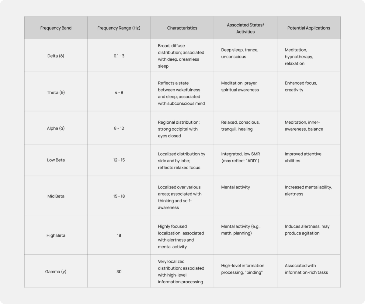
Unlocking Potential: Practical Applications
The rich tapestry of EEG frequency bands has practical applications that extend far beyond the realms of research. Cutting-edge technology now allows us to harness these waves for real-world use. Focus detection, calm detection, and concentration detection are just a few examples of how EEG data can be leveraged to enhance performance, well-being, and mental health.
How Nexstem helps?
Stream App's Bandpower Graph, which displays real-time EEG frequency band data, provides a powerful tool for monitoring brain activity in real-time. On the other hand, NexStem's WisdomAPI and WisdomSDK come equipped with advanced algorithms for Focus Detection, Emotion Detection, and Concentration, showcasing a comprehensive suite of capabilities for in-depth EEG data analysis.
This combination of real-time monitoring and advanced analytical tools sets a solid foundation for a wide range of applications in EEG research and development.
Did you know that it is possible to for a person to pass a lie detection test by exerting control over their physiological responses. Here we explore what would be an alternative to the common polygraph lie detection test using BCI technology.
Lie detection tests, often portrayed in movies as dramatic showdowns, are actually fascinating tools used in real-life scenarios. The most common method, the polygraph test, measures physiological responses like heart rate, blood pressure, and skin conductivity to assess truthfulness. While it's not foolproof and relies on the assumption that lying induces detectable physiological changes, it can be surprisingly accurate. The examiner sets the baseline by asking innocuous questions, then delves into the more critical queries. It's like a high-stakes game of poker, where involuntary reactions become the telltale signs. The results are akin to a puzzle for seasoned professionals, decoding the body's subtle cues to separate fact from fiction.
But there is a catch. It is possible for a person to potentially pass a lie detection test by exerting control over their physiological responses. This can be achieved through various techniques such as controlled breathing, mental distraction, or even the use of countermeasures like imagining stressful situations during baseline questions. Skilled individuals who are aware of these techniques may attempt to manipulate the results of the test. Additionally, some individuals may naturally exhibit limited physiological responses even when lying, making them more challenging to detect. So, despite its intriguing potential, lie detection tests aren't infallible and require skilled interpretation. They serve as one piece of the puzzle in investigations, reminding us that even in the quest for truth, human intuition and analysis remain paramount.
Electroencephalography (EEG)
It can be a more reliable alternative to polygraph tests. One may have semi-voluntary control over their physiological responses, but many internal mental responses are involuntary in nature. These responses can be reliably captured, and then recognized as patterns in EEG data. The P300 is one such pattern that can be used in lie-detection tests. All we need is a carefully designed environment, EEG recording setup, our prime suspect, and an invigilator - which could be another human or a simple computer program.
Picture P300 as your mental drum-roll, happening about 300 milliseconds after something catches your brain's eye. Now, here's the fun part: The brain throws this P300 party with a twist called the "oddball paradigm." It's like serving up a mix of familiar and surprise treats to your brain. When that surprise treat pops up, the P300 struts onto the scene, stealing the show with its snazzy moves! This P300 sensation isn't just for kicks though! It's your brain's secret agent, helping you focus on what really matters in a sea of distractions. It's like having a personal brain butler that whispers, "Hey, pay attention to this!"
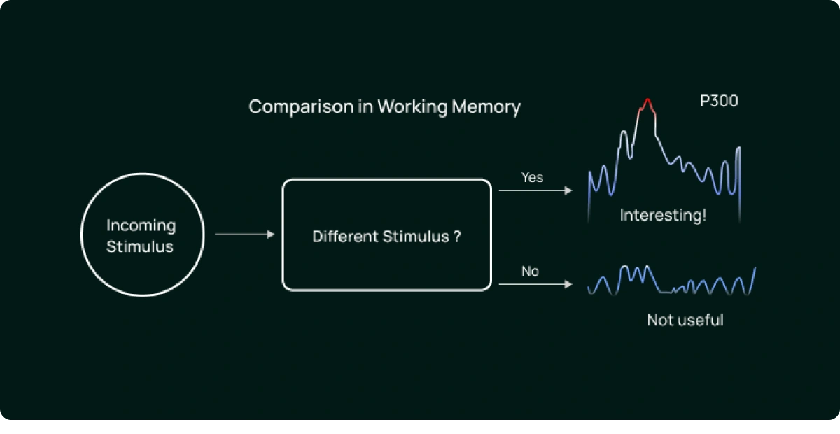
Role of P300 EEG Patterns
Let’s Imagine a scenario in a police investigation room to see how we can use P300 EEG patterns. Detective Anderson is questioning a suspect, John, about a recent burglary. John maintains his innocence, but Detective Anderson has reasons to suspect otherwise. This is where the P300, our cognitive truth-seeker, comes into play.
Detective Anderson has a set of statements related to the crime. Among them, there's one crucial statement he believes holds the truth: the location of a hidden stash of stolen goods. This statement is intermixed with other neutral statements to form a series.
John is instructed to respond truthfully to all statements. However, when he hears the statement about the hidden stash, he experiences a slight cognitive hiccup. This is because his brain, even though he's trying to hide it, recognizes the statement as relevant and unexpected. The P300, our lie-detecting superhero, picks up on this subtle brainwave pattern.
Meanwhile, electrodes placed on John's scalp are recording his brain activity. The EEG machine diligently captures the electrical signals generated by John's brain in response to each statement. When the statement about the hidden stash is presented, the P300 response emerges about 300 milliseconds later.
Detective Anderson, relying on the expertise of trained analysts and specialized software, examines the EEG data. They focus on the P300 response specifically, looking for distinct patterns that indicate heightened cognitive processing associated with the relevant statement.
In this case, the P300 signal corresponding to the statement about the hidden stash exhibits a stronger and more pronounced waveform compared to the neutral statements. This heightened P300 response is a telltale sign that John's brain recognizes the statement as important, suggesting he likely has knowledge of the hidden goods.
This crucial information becomes a powerful tool for Detective Anderson. While it doesn't serve as definitive proof of guilt, it provides a significant lead. It prompts further investigation, potentially leading to the recovery of the stolen items and strengthening the case against John.
Remember, this is a fictional scenario for illustrative purposes. In reality, things are not as simplistic. We would still need careful experimental design, scientific data analysis, and expert interpretation.
Current State of Research
A. Advancements in Signal Processing and Machine Learning
Researchers have made strides in refining signal processing techniques and applying machine learning algorithms to improve the accuracy and reliability of P300-based lie detection.
B. Integration with Multimodal Techniques
Combining EEG with other neuro-imaging methods (e.g., fMRI, eye-tracking) has shown promise in enhancing the accuracy of lie detection by providing complementary information.
C. Applied in Specific Contexts
P300-based lie detection has been explored in various domains, including criminal investigations, security screenings, and clinical assessments. It's important to note that it's not yet widely accepted for legal or forensic use in many jurisdictions.
D. BCIs and Assistive Technology
Beyond lie detection, the P300 has found applications in Brain-Computer Interfaces (BCIs), enabling individuals with motor disabilities to communicate or interact with their environment.
E. Potential Clinical Applications
P300-based research is extending into clinical areas, such as assessing cognitive functions in patients with brain injuries or neuro-degenerative disorders.
Challenges:
1. Individual Variability
Brainwave patterns can vary widely among individuals. This variability poses a challenge in developing a universal lie detection model that applies to all.
2. Ethical and Legal Considerations
The admissibility of P300-based lie detection in legal settings remains a subject of debate. False positives and negatives can have significant consequences, so ethical and legal frameworks must be carefully considered.
3. Real-World Context and Stress
Laboratory experiments may not fully capture the complexity and stress of real-world situations, where emotions, distractions, and high-stakes scenarios can influence results.
4. Interpretation of Results
While the P300 provides valuable information, interpreting its presence or absence requires expert knowledge and careful consideration of experimental design.
5. Cost and Accessibility
EEG equipment and expertise in analysis can be expensive and require specialized training, limiting the accessibility of P300-based lie detection methods.
6. Continual Technological Advancements
The field of EEG and lie detection is rapidly evolving. Keeping up with the latest technology and methodologies is crucial for accurate and reliable results.
In summary, while P300-based lie detection holds promise, it's not without its challenges. Ongoing research and advancements in technology, coupled with careful consideration of ethical and legal implications, are essential in moving this field forward.
Further reading:
- For deep dive into the P300 pattern -
The P300 Wave of the Human Event-Related Potential - P300 based lie detection-
Evaluation of P300 based Lie Detection Algorithm
P300 Based Deception Detection Using Convolutional Neural Networks
An experiment of lie detection based EEG-P300 classified by SVM algorithm - Other ways of lie detection using EEG-
Truth Identification from EEG Signal by using Convolution neural network: Lie Detection
Truth Identification from EEG Signal Using Frequency and Time Features with SVM Classifier