BCI Kickstarter #08 : Developing a Motor Imagery BCI: Controlling Devices with Your Mind
Welcome back to our BCI crash course! We've journeyed from the fundamental concepts of BCIs to the intricacies of brain signals, mastered the art of signal processing, and learned how to train intelligent algorithms to decode those signals. Now, we're ready to tackle a fascinating and powerful BCI paradigm: motor imagery. Motor imagery BCIs allow users to control devices simply by imagining movements. This technology holds immense potential for applications like controlling neuroprosthetics for individuals with paralysis, assisting in stroke rehabilitation, and even creating immersive gaming experiences. In this post, we'll guide you through the step-by-step process of building a basic motor imagery BCI using Python, MNE-Python, and scikit-learn. Get ready to harness the power of your thoughts to interact with technology!

Understanding Motor Imagery: The Brain's Internal Rehearsal
Before we dive into building our BCI, let's first understand the fascinating phenomenon of motor imagery.
What is Motor Imagery? Moving Without Moving
Motor imagery is the mental rehearsal of a movement without actually performing the physical action. It's like playing a video of the movement in your mind's eye, engaging the same neural processes involved in actual execution but without sending the final commands to your muscles.
Neural Basis of Motor Imagery: The Brain's Shared Representations
Remarkably, motor imagery activates similar brain regions and neural networks as actual movement. The motor cortex, the area of the brain responsible for planning and executing movements, is particularly active during motor imagery. This shared neural representation suggests that imagining a movement is a powerful way to engage the brain's motor system, even without physical action.
EEG Correlates of Motor Imagery: Decoding Imagined Movements
Motor imagery produces characteristic changes in EEG signals, particularly over the motor cortex. Two key features are:
- Event-Related Desynchronization (ERD): A decrease in power in specific frequency bands (mu, 8-12 Hz, and beta, 13-30 Hz) over the motor cortex during motor imagery. This decrease reflects the activation of neural populations involved in planning and executing the imagined movement.
- Event-Related Synchronization (ERS): An increase in power in those frequency bands after the termination of motor imagery, as the brain returns to its resting state.
These EEG features provide the foundation for decoding motor imagery and building BCIs that can translate imagined movements into control signals.
Building a Motor Imagery BCI: A Step-by-Step Guide
Now that we understand the neural basis of motor imagery, let's roll up our sleeves and build a BCI that can decode these imagined movements. We'll follow a step-by-step process, using Python, MNE-Python, and scikit-learn to guide us.
1. Loading the Dataset
Choosing the Dataset: BCI Competition IV Dataset 2a
For this project, we'll use the BCI Competition IV dataset 2a, a publicly available EEG dataset specifically designed for motor imagery BCI research. This dataset offers several advantages:
- Standardized Paradigm: The dataset follows a well-defined experimental protocol, making it easy to understand and replicate. Participants were instructed to imagine moving their left or right hand, providing clear labels for our classification task.
- Multiple Subjects: It includes recordings from nine subjects, providing a decent sample size to train and evaluate our BCI model.
- Widely Used: This dataset has been extensively used in BCI research, allowing us to compare our results with established benchmarks and explore various analysis approaches.
You can download the dataset from the BCI Competition IV website (http://www.bbci.de/competition/iv/).
Loading the Data: MNE-Python to the Rescue
Once you have the dataset downloaded, you can load it using MNE-Python's convenient functions. Here's a code snippet to get you started:
import mne
# Set the path to the dataset directory
data_path = '<path_to_dataset_directory>'
# Load the raw EEG data for subject 1
raw = mne.io.read_raw_gdf(data_path + '/A01T.gdf', preload=True)
Replace <path_to_dataset_directory> with the actual path to the directory where you've stored the dataset files. This code loads the data for subject "A01" from the training session ("T").
2. Data Preprocessing: Preparing the Signals for Decoding
Raw EEG data is often noisy and contains artifacts that can interfere with our analysis. Preprocessing is crucial for cleaning up the data and isolating the relevant brain signals associated with motor imagery.
Channel Selection: Focusing on the Motor Cortex
Since motor imagery primarily activates the motor cortex, we'll select EEG channels that capture activity from this region. Key channels include:
- C3: Located over the left motor cortex, sensitive to right-hand motor imagery.
- C4: Located over the right motor cortex, sensitive to left-hand motor imagery.
- Cz: Located over the midline, often used as a reference or to capture general motor activity.
# Select the desired channels
channels = ['C3', 'C4', 'Cz']
# Create a new raw object with only the selected channels
raw_selected = raw.pick_channels(channels)
Filtering: Isolating Mu and Beta Rhythms
We'll apply a band-pass filter to isolate the mu (8-12 Hz) and beta (13-30 Hz) frequency bands, as these rhythms exhibit the most prominent ERD/ERS patterns during motor imagery.
# Apply a band-pass filter from 8 Hz to 30 Hz
raw_filtered = raw_selected.filter(l_freq=8, h_freq=30)
This filtering step removes irrelevant frequencies and enhances the signal-to-noise ratio for detecting motor imagery-related brain activity.
Artifact Removal: Enhancing Data Quality (Optional)
Depending on the dataset and the quality of the recordings, we might need to apply artifact removal techniques. Independent Component Analysis (ICA) is particularly useful for identifying and removing artifacts like eye blinks, muscle activity, and heartbeats, which can contaminate our motor imagery signals. MNE-Python provides functions for performing ICA and visualizing the components, allowing us to select and remove those associated with artifacts. This step can significantly improve the accuracy and reliability of our motor imagery BCI.
3. Epoching and Visualizing: Zooming in on Motor Imagery
Now that we've preprocessed our EEG data, let's create epochs around the motor imagery cues, allowing us to focus on the brain activity specifically related to those imagined movements.
Defining Epochs: Capturing the Mental Rehearsal
The BCI Competition IV dataset 2a includes event markers indicating the onset of the motor imagery cues. We'll use these markers to create epochs, typically spanning a time window from a second before the cue to several seconds after it. This window captures the ERD and ERS patterns associated with motor imagery.
# Define event IDs for left and right hand motor imagery (refer to dataset documentation)
event_id = {'left_hand': 1, 'right_hand': 2}
# Set the epoch time window
tmin = -1 # 1 second before the cue
tmax = 4 # 4 seconds after the cue
# Create epochs
epochs = mne.Epochs(raw_filtered, events, event_id, tmin, tmax, baseline=(-1, 0), preload=True)
Baseline Correction: Removing Pre-Imagery Bias
We'll apply baseline correction to remove any pre-existing bias in the EEG signal, ensuring that our analysis focuses on the changes specifically related to motor imagery.
Visualizing: Inspecting and Gaining Insights
- Plotting Epochs: Use epochs.plot() to visualize individual epochs, inspecting for artifacts and observing the general patterns of brain activity during motor imagery.
- Topographical Maps: Use epochs['left_hand'].average().plot_topomap() and epochs['right_hand'].average().plot_topomap() to visualize the scalp distribution of mu and beta power changes during left and right hand motor imagery. These maps can help validate our channel selection and confirm that the ERD patterns are localized over the expected motor cortex areas.
4. Feature Extraction with Common Spatial Patterns (CSP): Maximizing Class Differences
Common Spatial Patterns (CSP) is a spatial filtering technique specifically designed to extract features that best discriminate between two classes of EEG data. In our case, these classes are left-hand and right-hand motor imagery.
Understanding CSP: Finding Optimal Spatial Filters
CSP seeks to find spatial filters that maximize the variance of one class while minimizing the variance of the other. It achieves this by solving an eigenvalue problem based on the covariance matrices of the two classes. The resulting spatial filters project the EEG data onto a new space where the classes are more easily separable
.
Applying CSP: MNE-Python's CSP Function
MNE-Python's mne.decoding.CSP() function makes it easy to extract CSP features:
from mne.decoding import CSP
# Create a CSP object
csp = CSP(n_components=4, reg=None, log=True, norm_trace=False)
# Fit the CSP to the epochs data
csp.fit(epochs['left_hand'].get_data(), epochs['right_hand'].get_data())
# Transform the epochs data using the CSP filters
X_csp = csp.transform(epochs.get_data())
Interpreting CSP Filters: Mapping Brain Activity
The CSP spatial filters represent patterns of brain activity that differentiate between left and right hand motor imagery. By visualizing these filters, we can gain insights into the underlying neural sources involved in these imagined movements.
Selecting CSP Components: Balancing Performance and Complexity
The n_components parameter in the CSP() function determines the number of CSP components to extract. Choosing the optimal number of components is crucial for balancing classification performance and model complexity. Too few components might not capture enough information, while too many can lead to overfitting. Cross-validation can help us find the optimal balance.
5. Classification with a Linear SVM: Decoding Motor Imagery
Choosing the Classifier: Linear SVM for Simplicity and Efficiency
We'll use a linear Support Vector Machine (SVM) to classify our motor imagery data. Linear SVMs are well-suited for this task due to their simplicity, efficiency, and ability to handle high-dimensional data. They seek to find a hyperplane that best separates the two classes in the feature space.
Training the Model: Learning from Spatial Patterns
from sklearn.svm import SVC
# Create a linear SVM classifier
svm = SVC(kernel='linear')
# Train the SVM model
svm.fit(X_csp_train, y_train)
Hyperparameter Tuning: Optimizing for Peak Performance
SVMs have hyperparameters, like the regularization parameter C, that control the model's complexity and generalization ability. Hyperparameter tuning, using techniques like grid search or cross-validation, helps us find the optimal values for these parameters to maximize classification accuracy.
Evaluating the Motor Imagery BCI: Measuring Mind Control
We've built our motor imagery BCI, but how well does it actually work? Evaluating its performance is crucial for understanding its capabilities and limitations, especially if we envision real-world applications.
Cross-Validation: Assessing Generalizability
To obtain a reliable estimate of our BCI's performance, we'll employ k-fold cross-validation. This technique helps us assess how well our model generalizes to unseen data, providing a more realistic measure of its real-world performance.
from sklearn.model_selection import cross_val_score
# Perform 5-fold cross-validation
scores = cross_val_score(svm, X_csp, y, cv=5)
# Print the average accuracy across the folds
print("Average accuracy: %0.2f" % scores.mean())
Performance Metrics: Beyond Simple Accuracy
- Accuracy: While accuracy, the proportion of correctly classified instances, is a useful starting point, it doesn't tell the whole story. For imbalanced datasets (where one class has significantly more samples than the other), accuracy can be misleading.
- Kappa Coefficient: The Kappa coefficient (κ) measures the agreement between the classifier's predictions and the true labels, taking into account the possibility of chance agreement. A Kappa value of 1 indicates perfect agreement, while 0 indicates agreement equivalent to chance. Kappa is a more robust metric than accuracy, especially for imbalanced datasets.
- Information Transfer Rate (ITR): ITR quantifies the amount of information transmitted by the BCI per unit of time, considering both accuracy and the number of possible choices. A higher ITR indicates a faster and more efficient communication system.
- Sensitivity and Specificity: These metrics provide a more nuanced view of classification performance. Sensitivity measures the proportion of correctly classified positive instances (e.g., correctly identifying left-hand imagery), while specificity measures the proportion of correctly classified negative instances (e.g., correctly identifying right-hand imagery).
Practical Implications: From Benchmarks to Real-World Use
Evaluating a motor imagery BCI goes beyond just looking at numbers. We need to consider the practical implications of its performance:
- Minimum Accuracy Requirements: Real-world applications often have minimum accuracy thresholds. For example, a neuroprosthetic controlled by a motor imagery BCI might require an accuracy of over 90% to ensure safe and reliable operation.
- User Experience: Beyond accuracy, factors like speed, ease of use, and mental effort also contribute to the overall user experience.
Unlocking the Potential of Motor Imagery BCIs
We've successfully built a basic motor imagery BCI, witnessing the power of EEG, signal processing, and machine learning to decode movement intentions directly from brain signals. Motor imagery BCIs hold immense potential for a wide range of applications, offering new possibilities for individuals with disabilities, stroke rehabilitation, and even immersive gaming experiences.
Resources for Further Reading
- Review article: EEG-Based Brain-Computer Interfaces Using Motor-Imagery: Techniques and Challenges https://www.ncbi.nlm.nih.gov/pmc/articles/PMC6471241/
- Review article: A review of critical challenges in MI-BCI: From conventional to deep learning methods https://www.sciencedirect.com/science/article/abs/pii/S016502702200262X
- BCI Competition IV Dataset 2a https://www.bbci.de/competition/iv/desc_2a.pdf
From Motor Imagery to Advanced BCI Paradigms
This concludes our exploration of building a motor imagery BCI. You've gained valuable insights into the neural basis of motor imagery, learned how to extract features using CSP, trained a classifier to decode movement intentions, and evaluated the performance of your BCI model.
In our final blog post, we'll explore the exciting frontier of advanced BCI paradigms and future directions. We'll delve into concepts like hybrid BCIs, adaptive algorithms, ethical considerations, and the ever-expanding possibilities that lie ahead in the world of brain-computer interfaces. Stay tuned for a glimpse into the future of mind-controlled technology!

Capturing a biosignal is only the beginning. The real challenge starts once those tiny electrical fluctuations from your brain, heart, or muscles are recorded. What do they mean? How do we clean, interpret, and translate them into something both the machine and eventually we can understand? In this blog, we move beyond sensors to the invisible layer of algorithms and analysis that turns raw biosignal data into insight. From filtering and feature extraction to machine learning and real-time interpretation, this is how your body’s electrical language becomes readable.
Every heartbeat, every blink, every neural spark produces a complex trace of electrical or mechanical activity. These traces known collectively as biosignals are the raw currency of human-body intelligence. But in their raw form they’re noisy, dynamic, and difficult to interpret.
The transformation from raw sensor output to interpreted understanding is what we call biosignal processing. It’s the foundation of modern neuro- and bio-technology, enabling everything from wearable health devices to brain-computer interfaces (BCIs).
The Journey: From Raw Signal to Insight
When a biosignal sensor records, it captures a continuous stream of data—voltage fluctuations (in EEG, ECG, EMG), optical intensity changes, or pressure variations.
But that stream is messy. It includes baseline drift, motion artefacts, impedance shifts as electrodes dry, physiological artefacts (eye blinks, swallowing, jaw tension), and environmental noise (mains hum, electromagnetic interference).
Processing converts this noise-ridden stream into usable information, brain rhythms, cardiac cycles, muscle commands, or stress patterns.
Stage 1: Pre-processing — Cleaning the Signal
Before we can make sense of the body’s signals, we must remove the noise.
- Filtering: Band-pass filters (typically 0.5–45 Hz for EEG) remove slow drift and high-frequency interference; notch filters suppress 50/60 Hz mains hum.
- Artifact removal: Independent Component Analysis (ICA) and regression remain the most common methods for removing eye-blink (EOG) and muscle (EMG) artefacts, though hybrid and deep learning–based techniques are becoming more popular for automated denoising.
- Segmentation / epoching: Continuous biosignals are divided into stable time segments—beat-based for ECG or fixed/event-locked windows for EEG (e.g., 250 ms–1 s)—to capture temporal and spectral features more reliably.
- Normalization & baseline correction: Normalization rescales signal amplitudes across channels or subjects, while baseline correction removes constant offsets or drift to align signals to a common reference.
Think of this stage as cleaning a lens: if you don’t remove the smudges, everything you see through it will be distorted.
Stage 2: Feature Extraction — Finding the Patterns
Once the signal is clean, we quantify its characteristics, features that encode physiological or cognitive states.
Physiological Grounding
- EEG: Arises from synchronized postsynaptic currents in cortical pyramidal neurons.
- EMG: Records summed action potentials from contracting muscle fibers.
- ECG: Reflects rhythmic depolarization of cardiac pacemaker (SA node) cells.
Time-domain Features
Mean, variance, RMS, and zero-crossing rate quantify signal amplitude and variability over time. In EMG, Mean Absolute Value (MAV) and Waveform Length (WL) reflect overall muscle activation and fatigue progression.
Frequency & Spectral Features
The power of each EEG band tends to vary systematically across mental states.

Time–Frequency & Non-Linear Features
Wavelet transforms or Empirical Mode Decomposition capture transient events. Entropy- and fractal-based measures reveal complexity, useful for fatigue or cognitive-load studies.
Spatial Features
For multi-channel EEG, spatial filters such as Common Spatial Patterns (CSP) isolate task-specific cortical sources.
Stage 3: Classification & Machine Learning — Teaching Machines to Read the Body
After feature extraction, machine-learning models map those features to outcomes: focused vs fatigued, gesture A vs gesture B, normal vs arrhythmic.
- Classical ML: SVM, LDA, Random Forest , effective for curated features.
- Deep Learning: CNNs, LSTMs, Graph CNNs , learn directly from raw or minimally processed data.
- Transfer Learning: Improves cross-subject performance by adapting pretrained networks.
- Edge Inference: Deploying compact models (TinyML, quantized CNNs) on embedded hardware to achieve < 10 ms latency.
This is where raw physiology becomes actionable intelligence.
Interpreting Results — Making Sense of the Numbers
A robust pipeline delivers meaning, not just data:
- Detecting stress or fatigue for adaptive feedback.
- Translating EEG patterns into commands for prosthetics or interfaces.
- Monitoring ECG spectral shifts to flag early arrhythmias.
- Quantifying EMG coordination for rehabilitation or athletic optimization.
Performance hinges on accuracy, latency, robustness, and interpretability, especially when outcomes influence safety-critical systems.
Challenges and Future Directions
Technical: Inter-subject variability, electrode drift, real-world noise, and limited labeled datasets still constrain accuracy.
Ethical / Explainability: As algorithms mediate more decisions, transparency and consent are non-negotiable.
Multimodal Fusion: Combining EEG + EMG + ECG data improves reliability but raises synchronization and power-processing challenges.
Edge AI & Context Awareness: The next frontier is continuous, low-latency interpretation that adapts to user state and environment in real time.
Final Thought
Capturing a biosignal is only half the story. What truly powers next-gen neurotech and human-aware systems is turning that signal into sense. From electrodes and photodiodes to filters and neural nets, each link in this chain brings us closer to devices that don’t just measure humans; they understand them.
Every thought, heartbeat, and muscle twitch leaves behind a signal, but how do we actually capture them? In this blog post, we explore the sensors that make biosignal measurement possible, from EEG and ECG electrodes to optical and biochemical interfaces, and what it takes to turn those signals into meaningful data.
When we think of sensors, we often imagine cameras, microphones, or temperature gauges. But some of the most fascinating sensors aren’t designed to measure the world, they’re designed to measure you.
These are biosignal sensors: tiny, precise, and increasingly powerful tools that decode the electrical whispers of your brain, heart, and muscles. They're the hidden layer enabling brain-computer interfaces, wearables, neurofeedback systems, and next-gen health diagnostics.
But how do they actually work? And what makes one sensor better than another?
Let’s break it down, from scalp to circuit board.
First, a Quick Recap: What Are Biosignals?
Biosignals are the body’s internal signals, electrical, optical, or chemical , that reflect brain activity, heart function, muscle movement, and more. If you’ve read our earlier post on biosignal types, you’ll know they’re the raw material for everything from brain-computer interfaces to biometric wearables.
In this blog, we shift focus to the devices and sensors that make it possible to detect these signals in the real world, and what it takes to do it well.
The Devices That Listen In: Biosignal Sensor Types
.webp)
A Closer Look: How These Sensors Work
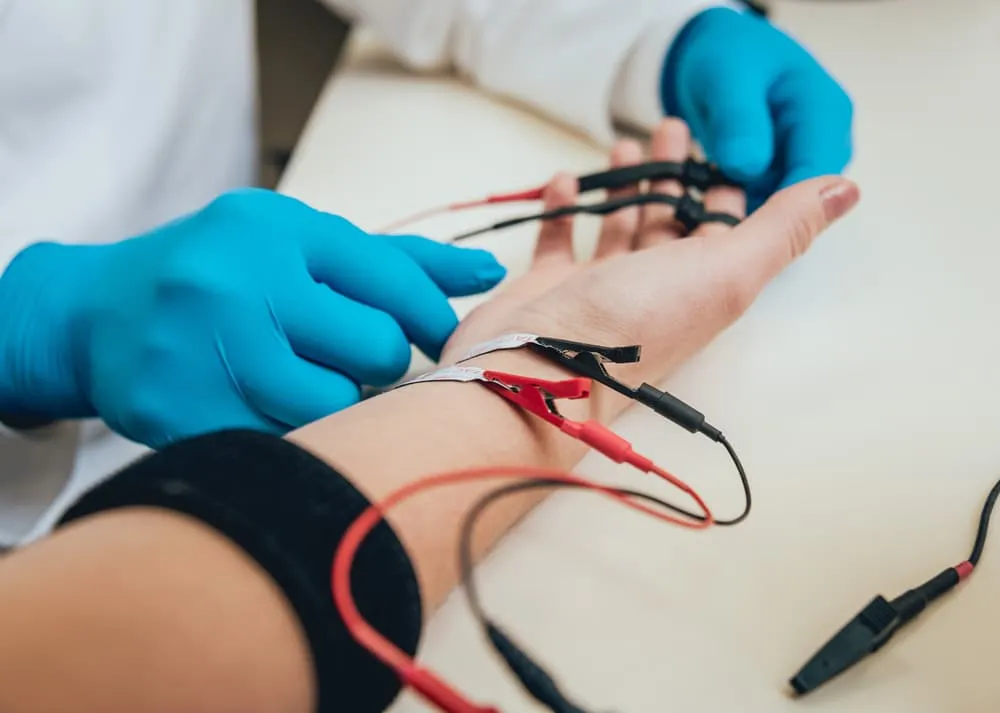
1. EEG / ECG / EMG – Electrical Sensors
These measure voltage fluctuations at the skin surface, caused by underlying bioelectric activity.
It’s like trying to hear a whisper in a thunderstorm; brain and muscle signals are tiny, and will get buried under noise unless the electrodes make solid contact and the amplifier filters aggressively.
There are two key electrode types:
- Wet electrodes: Use conductive gel or Saline for better signal quality. Still the gold standard in labs.
- Dry electrodes: More practical for wearables but prone to motion artifacts and noise (due to higher electrode resistance).
Signal acquisition often involves differential recording and requires high common-mode rejection ratios (CMRR) to suppress environmental noise.
Fun Fact: Even blinking your eyes generates an EMG signal that can overwhelm EEG data. That’s why artifact rejection algorithms are critical in EEG-based systems.
2. Optical Sensors (PPG, fNIRS)
These use light to infer blood flow or oxygenation levels:
- PPG: Emits light into the skin and measures reflection, pulsatile blood flow alters absorption.
- fNIRS: Uses near-infrared light to differentiate oxygenated vs. deoxygenated hemoglobin in the cortex.
Example: Emerging wearable fNIRS systems like Kernel Flow and OpenBCI Galea are making brain oxygenation measurement accessible outside labs.
3. Galvanic Skin Response / EDA – Emotion’s Electrical Signature
GSR (also called electrodermal activity) sensors detect subtle changes in skin conductance caused by sweat gland activity, a direct output of sympathetic nervous system arousal. When you're stressed or emotionally engaged, your skin becomes more conductive, and GSR sensors pick that up.
These sensors apply a small voltage across two points on the skin and track resistance over time. They're widely used in emotion tracking, stress monitoring, and psychological research due to their simplicity and responsiveness.
Together, these sensors form the foundation of modern biosignal acquisition — but capturing clean signals isn’t just about what you use, it’s about how you use it.
How Signal Quality Is Preserved
Measurement is just step one; capturing clean, interpretable signals involves:
- Analog Front End (AFE): Amplifies low signals while rejecting noise.
- ADC: Converts continuous analog signals into digital data.
- Signal Conditioning: Filters out drift, DC offset, 50/60Hz noise.
- Artifact Removal: Eye blinks, jaw clenches, muscle twitches.
Hardware platforms like TI’s ADS1299 and Analog Devices’ MAX30003 are commonly used in EEG and ECG acquisition systems.
New Frontiers in Biosignal Measurement
- Textile Sensors: Smart clothing with embedded electrodes for long-term monitoring.
- Biochemical Sensors: Detect metabolites like lactate, glucose, or cortisol in sweat or saliva.
- Multimodal Systems: Combining EEG + EMG + IMU + PPG in unified setups to boost accuracy.
A recent study involving transradial amputees demonstrated that combining EEG and EMG signals via a transfer learning model increased classification accuracy by 2.5–4.3% compared to EEG-only models.
Other multimodal fusion approaches, such as combining EMG and force myography (FMG), have shown classification improvements of over 10% compared to EMG alone.
Why Should You Care?
Because how we measure determines what we understand, and what we can build.
Whether it's a mental wellness wearable, a prosthetic limb that responds to thought, or a personalized neurofeedback app, it all begins with signal integrity. Bad data means bad decisions. Good signals? They unlock new frontiers.
Final Thought
We’re entering an era where technology doesn’t just respond to clicks, it responds to cognition, physiology, and intent.
Biosignal sensors are the bridge. Understanding them isn’t just for engineers; it’s essential for anyone shaping the future of human-aware tech.

In our previous blog, we explored how biosignals serve as the body's internal language—electrical, mechanical, and chemical messages that allow us to understand and interface with our physiology. Among these, electrical biosignals are particularly important for understanding how our nervous system, muscles, and heart function in real time. In this article, we’ll take a closer look at three of the most widely used electrical biosignals—EEG, ECG, and EMG—and their growing role in neurotechnology, diagnostics, performance tracking, and human-computer interaction. If you're new to the concept of biosignals, you might want to check out our introductory blog for a foundational overview.
"The body is a machine, and we must understand its currents if we are to understand its functions."-Émil du Bois-Reymond, pioneer in electrophysiology.
Life, though rare in the universe, leaves behind unmistakable footprints—biosignals. These signals not only confirm the presence of life but also narrate what a living being is doing, feeling, or thinking. As technology advances, we are learning to listen to these whispers of biology. Whether it’s improving health, enhancing performance, or building Brain-Computer Interfaces (BCIs), understanding biosignals is key.
Among the most studied biosignals are:
- Electroencephalogram (EEG) – from the brain
- Electrocardiogram (ECG) – from the heart
- Electromyogram (EMG) – from muscles
- Galvanic Skin Response (GSR) – from skin conductance
These signals are foundational for biosignal processing, real-time monitoring, and interfacing the human body with machines. In this article we look at some of these biosignals and some fascinating stories behind them.
Electroencephalography (EEG): Listening to Brainwaves
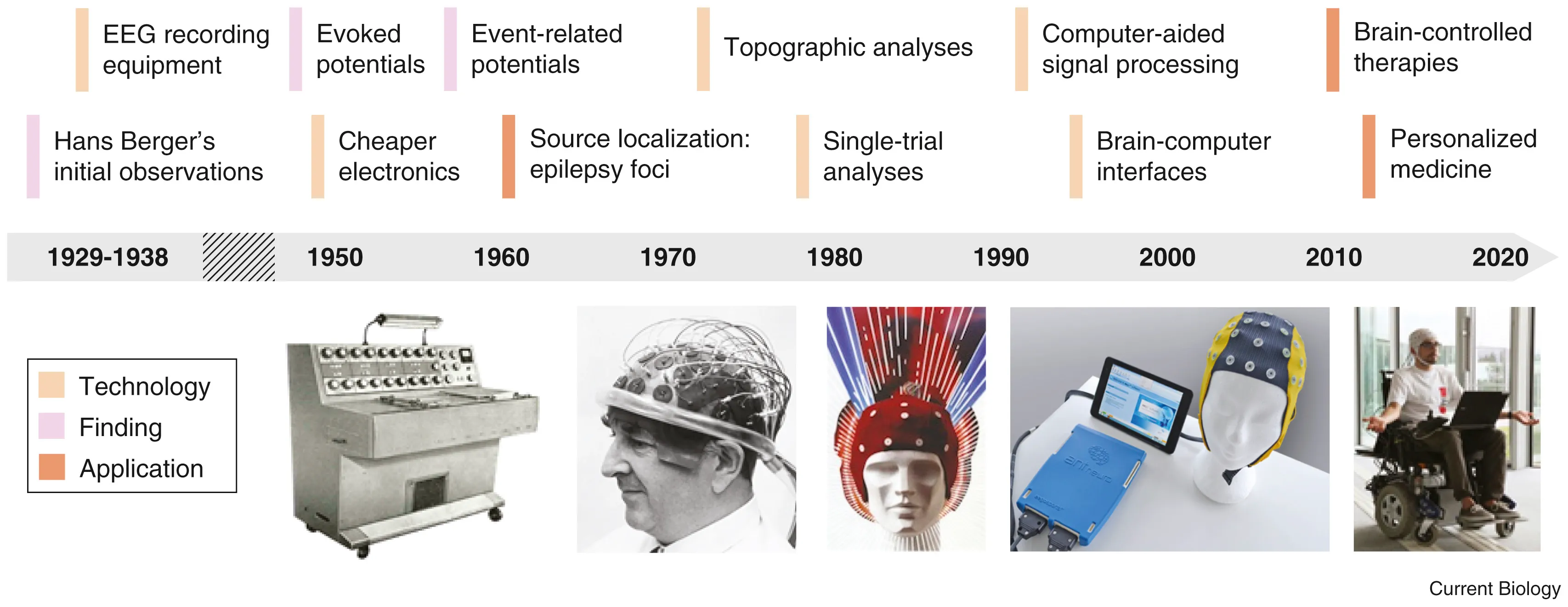
In 1893, a 19 year old Hans Berger fell from a horse and had a near death experience. Little did he know that it would be a pivotal moment in the history of neurotechnology. The same day he received a telegram from his sister who was extremely concerned for him because she had a bad feeling. Hans Berger was convinced that this was due to the phenomenon of telepathy. After all, it was the age of radio waves, so why can’t there be “brain waves”? In his ensuing 30 year career telepathy was not established but in his pursuit, Berger became the first person to record brain waves.
When neurons fire together, they generate tiny electrical currents. These can be recorded using electrodes placed on the scalp (EEG), inside the skull (intracranial EEG), or directly on the brain (ElectroCorticogram). EEG signal processing is used not only to understand the brain’s rhythms but also in EEG-based BCI systems, allowing communication and control for people with paralysis. Event-Related Potentials (ERPs) and Local Field Potentials (LFPs) are specialized types of EEG signals that provide insights into how the brain responds to specific stimuli.
Electrocardiogram (ECG): The Rhythm of the Heart
The heart has its own internal clock which produces tiny electrical signals every time it beats. Each heartbeat starts with a small electrical impulse made by a special part of the heart called the sinoatrial (SA) node. This impulse spreads through the heart muscle and makes it contract, first the upper (atria) and then lower chambers (ventricles) – that’s what pumps blood. This process produces voltage changes, which can be recorded via electrodes on the skin.
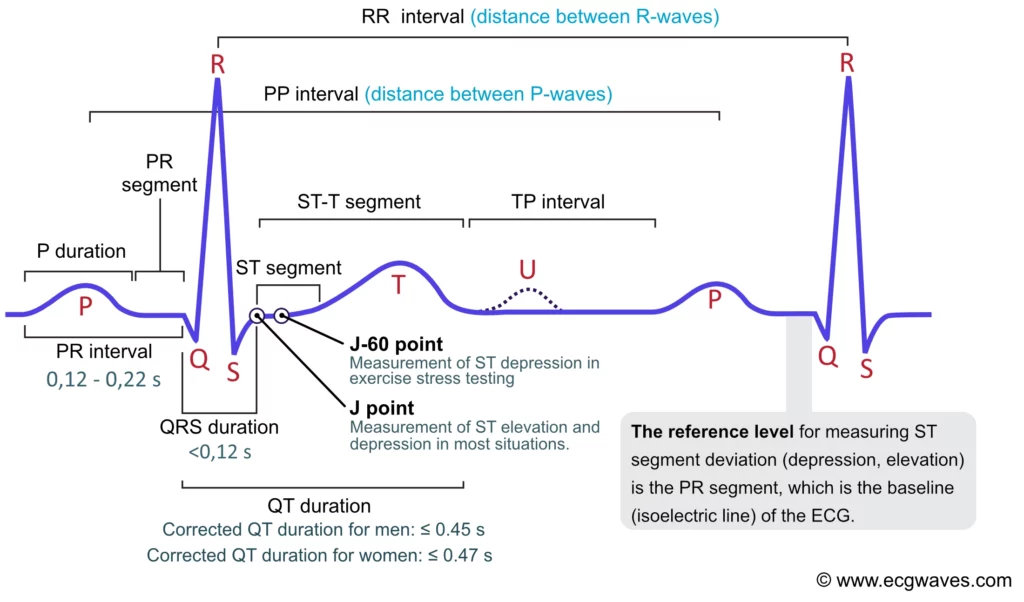
This gives rise to the classic PQRST waveform, with each component representing a specific part of the heart’s cycle. Modern wearables and medical devices use ECG signal analysis to monitor heart health in real time.
Fun fact: The waveform starts with “P” because Willem Einthoven left room for earlier letters—just in case future scientists discovered pre-P waves! So, thanks to a cautious scientist, we have the quirky naming system we still follow today.
Electromyography (EMG): The Language of Movement
When we perform any kind of movement - lifting our arm, kicking our leg, smiling, blinking or even breathing- our brain sends electrical signals to our muscles telling them to contract. When these neurons, known as motor neurons fire they release electrical impulses that travel to the muscle, causing it to contract. This electrical impulse—called a motor unit action potential (MUAP)—is what we see as an EMG signal. So, every time we move, we are generating an EMG signal!
Medical Applications
Medically, EMG is used for monitoring muscle fatigue especially in rehabilitation settings and muscle recovery post-injury or surgery. This helps clinicians measure progress and optimize therapy. EMG can distinguish between voluntary and involuntary movements, making it useful in diagnosing neuromuscular disorders, assessing stroke recovery, spinal cord injuries, and motor control dysfunctions.
Performance and Sports Science
In sports science, EMG can tell us muscle-activation timing and quantify force output of muscle groups. These are important factors to measure performance improvement in any sport. The number of motor units recruited and the synergy between muscle groups, helps us capture “mind-muscle connection” and muscle memory. Such things which were previously spoken off in a figurative manner can be scientifically measured and quantified using EMG. By tracking these parameters we get a window into movement efficiency and athletic performance. EMG is also used for biofeedback training, enabling individuals to consciously correct poor movement habits or retrain specific muscles
Beyond medicine and sports, EMG is used for gesture recognition in AR/VR and gaming, silent speech detection via facial EMG, and next-gen prosthetics and wearable exosuits that respond to the user’s muscle signals. EMG can be used in brain-computer interfaces (BCIs), helping paralyzed individuals control digital devices or communicate through subtle muscle activity. EMG bridges the gap between physiology, behavior, and technology—making it a critical tool in healthcare, performance optimization, and human-machine interaction.
As biosignal processing becomes more refined and neurotech devices more accessible, we are moving toward a world where our body speaks—and machines understand. Whether it’s detecting the subtlest brainwaves, tracking a racing heart, or interpreting muscle commands, biosignals are becoming the foundation of the next digital revolution. One where technology doesn’t just respond, but understands.