The impact of musical training on the adult brain

Learning to play a musical instrument not only enhances your musical skills but also reshapes the adult brain. Discover how musical training bridges nature and nurture, transforming both brain structure and function.
Music has long been known to have a profound impact on our emotions and well-being. But did you know that learning to play a musical instrument can also shape the adult brain? In a recent review article, researchers delve into the structural and functional differences between the brains of musicians and non-musicians, shedding light on the fascinating effects of musical training.

Nature vs. Nurture: Predispositions or Training?

One of the key questions in this inquiry is whether the observed differences between musicians and non-musicians are due to inherent predispositions or the result of training. Recent research explores brain reorganization and neuronal markers related to learning to play a musical instrument. Turns out, the "musical brain" is influenced by both natural human neurodiversity and training practice.

Structural and Functional Differences

There are structural and functional differences between the brains of musicians and non-musicians. Specifically, regions associated with motor control and auditory processing show notable disparities. These differences suggest that musical training can lead to specific adaptations in these brain areas, potentially enhancing motor skills and auditory perception.

Impact on the Motor Network and Auditory System

Longitudinal studies have demonstrated that music training can induce functional changes in the motor network and its connectivity with the auditory system. This finding suggests that learning to play an instrument not only refines motor control but also strengthens the integration between auditory and motor processes. Such cross-modal plasticity may contribute to musicians' exceptional ability to synchronize their movements with sound.
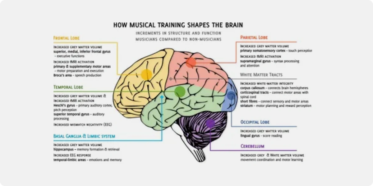
How musical training shapes the brain

Predictors of Musical Learning Success

Research has also found potential predictors of musical learning success. Specific brain activation patterns and functional connectivity are possible indicators of an individual's aptitude for musical training. These findings open up exciting possibilities for personalized approaches to music education, allowing educators to tailor instruction to each student's unique neural profile.

Some generic predictors, however, are:

Attitude and Motivation

Positive attitudes towards the music being learned and high motivational levels have emerged as significant predictors of musical learning success. Individuals displaying enthusiasm and a receptive mindset exhibit enhanced learning outcomes, underscoring the importance of psychological factors in the musical learning process.

Intelligence

General intelligence demonstrates a positive correlation with musical skill acquisition, suggesting that cognitive aptitude plays a pivotal role in mastering musical elements. This finding underscores the cognitive demands of musical learning and emphasizes the relevance of intelligence as a predictor of success in this domain.

Reward and Pleasure

The level of liking or enjoyment of a particular piece of music before training has been identified as a critical predictor influencing the ability to learn and achieve proficiency. The intrinsic reward and pleasure associated with musical engagement contribute to heightened receptivity and commitment to the learning process.

Music Predictability

Musical predictability emerges as a noteworthy factor influencing pupil dilation and promoting motor learning in non-musicians. The predictability of musical elements contributes to a more efficient cognitive processing of auditory information, enhancing the overall learning experience.

In conclusion, musical training has transformative effects on the adult brain. The differences observed between musicians and non-musicians are likely a result of a combination of innate predispositions and training practice, and understanding these neural adaptations can inform educational strategies and promote the benefits of music in cognitive development and overall well-being

Explore other blogs
BCI Kickstarter
BCI Kickstarter #08 : Developing a Motor Imagery BCI: Controlling Devices with Your Mind

Welcome back to our BCI crash course! We've journeyed from the fundamental concepts of BCIs to the intricacies of brain signals, mastered the art of signal processing, and learned how to train intelligent algorithms to decode those signals. Now, we're ready to tackle a fascinating and powerful BCI paradigm: motor imagery. Motor imagery BCIs allow users to control devices simply by imagining movements. This technology holds immense potential for applications like controlling neuroprosthetics for individuals with paralysis, assisting in stroke rehabilitation, and even creating immersive gaming experiences. In this post, we'll guide you through the step-by-step process of building a basic motor imagery BCI using Python, MNE-Python, and scikit-learn. Get ready to harness the power of your thoughts to interact with technology!

by
Team Nexstem

Understanding Motor Imagery: The Brain's Internal Rehearsal

Before we dive into building our BCI, let's first understand the fascinating phenomenon of motor imagery.

What is Motor Imagery? Moving Without Moving

Motor imagery is the mental rehearsal of a movement without actually performing the physical action.  It's like playing a video of the movement in your mind's eye, engaging the same neural processes involved in actual execution but without sending the final commands to your muscles.

Neural Basis of Motor Imagery: The Brain's Shared Representations

Remarkably, motor imagery activates similar brain regions and neural networks as actual movement.  The motor cortex, the area of the brain responsible for planning and executing movements, is particularly active during motor imagery. This shared neural representation suggests that imagining a movement is a powerful way to engage the brain's motor system, even without physical action.

EEG Correlates of Motor Imagery: Decoding Imagined Movements

Motor imagery produces characteristic changes in EEG signals, particularly over the motor cortex.  Two key features are:

  • Event-Related Desynchronization (ERD): A decrease in power in specific frequency bands (mu, 8-12 Hz, and beta, 13-30 Hz) over the motor cortex during motor imagery. This decrease reflects the activation of neural populations involved in planning and executing the imagined movement.
  • Event-Related Synchronization (ERS):  An increase in power in those frequency bands after the termination of motor imagery, as the brain returns to its resting state.

These EEG features provide the foundation for decoding motor imagery and building BCIs that can translate imagined movements into control signals.

Building a Motor Imagery BCI: A Step-by-Step Guide

Now that we understand the neural basis of motor imagery, let's roll up our sleeves and build a BCI that can decode these imagined movements.  We'll follow a step-by-step process, using Python, MNE-Python, and scikit-learn to guide us.

1. Loading the Dataset

Choosing the Dataset: BCI Competition IV Dataset 2a

For this project, we'll use the BCI Competition IV dataset 2a, a publicly available EEG dataset specifically designed for motor imagery BCI research. This dataset offers several advantages:

  • Standardized Paradigm: The dataset follows a well-defined experimental protocol, making it easy to understand and replicate. Participants were instructed to imagine moving their left or right hand, providing clear labels for our classification task.
  • Multiple Subjects: It includes recordings from nine subjects, providing a decent sample size to train and evaluate our BCI model.
  • Widely Used:  This dataset has been extensively used in BCI research, allowing us to compare our results with established benchmarks and explore various analysis approaches.

You can download the dataset from the BCI Competition IV website (http://www.bbci.de/competition/iv/).

Loading the Data: MNE-Python to the Rescue

Once you have the dataset downloaded, you can load it using MNE-Python's convenient functions.  Here's a code snippet to get you started:

import mne

# Set the path to the dataset directory

data_path = '<path_to_dataset_directory>'

# Load the raw EEG data for subject 1

raw = mne.io.read_raw_gdf(data_path + '/A01T.gdf', preload=True)

Replace <path_to_dataset_directory> with the actual path to the directory where you've stored the dataset files.  This code loads the data for subject "A01" from the training session ("T").

2. Data Preprocessing: Preparing the Signals for Decoding

Raw EEG data is often noisy and contains artifacts that can interfere with our analysis.  Preprocessing is crucial for cleaning up the data and isolating the relevant brain signals associated with motor imagery.

Channel Selection: Focusing on the Motor Cortex

Since motor imagery primarily activates the motor cortex, we'll select EEG channels that capture activity from this region.  Key channels include:

  • C3: Located over the left motor cortex, sensitive to right-hand motor imagery.
  • C4:  Located over the right motor cortex, sensitive to left-hand motor imagery.
  • Cz:  Located over the midline, often used as a reference or to capture general motor activity.

# Select the desired channels

channels = ['C3', 'C4', 'Cz']

# Create a new raw object with only the selected channels

raw_selected = raw.pick_channels(channels)

Filtering:  Isolating Mu and Beta Rhythms

We'll apply a band-pass filter to isolate the mu (8-12 Hz) and beta (13-30 Hz) frequency bands, as these rhythms exhibit the most prominent ERD/ERS patterns during motor imagery.

# Apply a band-pass filter from 8 Hz to 30 Hz

raw_filtered = raw_selected.filter(l_freq=8, h_freq=30)

This filtering step removes irrelevant frequencies and enhances the signal-to-noise ratio for detecting motor imagery-related brain activity.

Artifact Removal: Enhancing Data Quality (Optional)

Depending on the dataset and the quality of the recordings, we might need to apply artifact removal techniques.  Independent Component Analysis (ICA) is particularly useful for identifying and removing artifacts like eye blinks, muscle activity, and heartbeats, which can contaminate our motor imagery signals.  MNE-Python provides functions for performing ICA and visualizing the components, allowing us to select and remove those associated with artifacts.  This step can significantly improve the accuracy and reliability of our motor imagery BCI.

3. Epoching and Visualizing: Zooming in on Motor Imagery

Now that we've preprocessed our EEG data, let's create epochs around the motor imagery cues, allowing us to focus on the brain activity specifically related to those imagined movements.

Defining Epochs: Capturing the Mental Rehearsal

The BCI Competition IV dataset 2a includes event markers indicating the onset of the motor imagery cues.  We'll use these markers to create epochs, typically spanning a time window from a second before the cue to several seconds after it.  This window captures the ERD and ERS patterns associated with motor imagery.

# Define event IDs for left and right hand motor imagery (refer to dataset documentation)

event_id = {'left_hand': 1, 'right_hand': 2}

# Set the epoch time window

tmin = -1  # 1 second before the cue

tmax = 4   # 4 seconds after the cue

# Create epochs

epochs = mne.Epochs(raw_filtered, events, event_id, tmin, tmax, baseline=(-1, 0), preload=True)

Baseline Correction:  Removing Pre-Imagery Bias

We'll apply baseline correction to remove any pre-existing bias in the EEG signal, ensuring that our analysis focuses on the changes specifically related to motor imagery.

Visualizing: Inspecting and Gaining Insights

  • Plotting Epochs:  Use epochs.plot() to visualize individual epochs, inspecting for artifacts and observing the general patterns of brain activity during motor imagery.
  • Topographical Maps:  Use epochs['left_hand'].average().plot_topomap() and epochs['right_hand'].average().plot_topomap() to visualize the scalp distribution of mu and beta power changes during left and right hand motor imagery. These maps can help validate our channel selection and confirm that the ERD patterns are localized over the expected motor cortex areas.

4. Feature Extraction with Common Spatial Patterns (CSP): Maximizing Class Differences

Common Spatial Patterns (CSP) is a spatial filtering technique specifically designed to extract features that best discriminate between two classes of EEG data. In our case, these classes are left-hand and right-hand motor imagery.

Understanding CSP: Finding Optimal Spatial Filters

CSP seeks to find spatial filters that maximize the variance of one class while minimizing the variance of the other. It achieves this by solving an eigenvalue problem based on the covariance matrices of the two classes. The resulting spatial filters project the EEG data onto a new space where the classes are more easily separable
.

Applying CSP: MNE-Python's CSP Function

MNE-Python's mne.decoding.CSP() function makes it easy to extract CSP features:

from mne.decoding import CSP

# Create a CSP object

csp = CSP(n_components=4, reg=None, log=True, norm_trace=False)

# Fit the CSP to the epochs data

csp.fit(epochs['left_hand'].get_data(), epochs['right_hand'].get_data())

# Transform the epochs data using the CSP filters

X_csp = csp.transform(epochs.get_data())

Interpreting CSP Filters: Mapping Brain Activity

The CSP spatial filters represent patterns of brain activity that differentiate between left and right hand motor imagery.  By visualizing these filters, we can gain insights into the underlying neural sources involved in these imagined movements.

Selecting CSP Components: Balancing Performance and Complexity

The n_components parameter in the CSP() function determines the number of CSP components to extract.  Choosing the optimal number of components is crucial for balancing classification performance and model complexity.  Too few components might not capture enough information, while too many can lead to overfitting. Cross-validation can help us find the optimal balance.

5. Classification with a Linear SVM: Decoding Motor Imagery

Choosing the Classifier: Linear SVM for Simplicity and Efficiency

We'll use a linear Support Vector Machine (SVM) to classify our motor imagery data.  Linear SVMs are well-suited for this task due to their simplicity, efficiency, and ability to handle high-dimensional data.  They seek to find a hyperplane that best separates the two classes in the feature space.

Training the Model: Learning from Spatial Patterns

from sklearn.svm import SVC

# Create a linear SVM classifier

svm = SVC(kernel='linear')

# Train the SVM model

svm.fit(X_csp_train, y_train)

Hyperparameter Tuning: Optimizing for Peak Performance

SVMs have hyperparameters, like the regularization parameter C, that control the model's complexity and generalization ability.  Hyperparameter tuning, using techniques like grid search or cross-validation, helps us find the optimal values for these parameters to maximize classification accuracy.

Evaluating the Motor Imagery BCI: Measuring Mind Control

We've built our motor imagery BCI, but how well does it actually work? Evaluating its performance is crucial for understanding its capabilities and limitations, especially if we envision real-world applications.

Cross-Validation: Assessing Generalizability

To obtain a reliable estimate of our BCI's performance, we'll employ k-fold cross-validation.  This technique helps us assess how well our model generalizes to unseen data, providing a more realistic measure of its real-world performance.

from sklearn.model_selection import cross_val_score

# Perform 5-fold cross-validation

scores = cross_val_score(svm, X_csp, y, cv=5)

# Print the average accuracy across the folds

print("Average accuracy: %0.2f" % scores.mean())

Performance Metrics: Beyond Simple Accuracy

  • Accuracy: While accuracy, the proportion of correctly classified instances, is a useful starting point, it doesn't tell the whole story.  For imbalanced datasets (where one class has significantly more samples than the other), accuracy can be misleading.
  • Kappa Coefficient: The Kappa coefficient (κ) measures the agreement between the classifier's predictions and the true labels, taking into account the possibility of chance agreement.  A Kappa value of 1 indicates perfect agreement, while 0 indicates agreement equivalent to chance. Kappa is a more robust metric than accuracy, especially for imbalanced datasets.
  • Information Transfer Rate (ITR): ITR quantifies the amount of information transmitted by the BCI per unit of time, considering both accuracy and the number of possible choices.  A higher ITR indicates a faster and more efficient communication system.
  • Sensitivity and Specificity:  These metrics provide a more nuanced view of classification performance.  Sensitivity measures the proportion of correctly classified positive instances (e.g., correctly identifying left-hand imagery), while specificity measures the proportion of correctly classified negative instances (e.g., correctly identifying right-hand imagery).

Practical Implications: From Benchmarks to Real-World Use

Evaluating a motor imagery BCI goes beyond just looking at numbers.  We need to consider the practical implications of its performance:

  • Minimum Accuracy Requirements:  Real-world applications often have minimum accuracy thresholds.  For example, a neuroprosthetic controlled by a motor imagery BCI might require an accuracy of over 90% to ensure safe and reliable operation.
  • User Experience:  Beyond accuracy, factors like speed, ease of use, and mental effort also contribute to the overall user experience.

Unlocking the Potential of Motor Imagery BCIs

We've successfully built a basic motor imagery BCI, witnessing the power of EEG, signal processing, and machine learning to decode movement intentions directly from brain signals. Motor imagery BCIs hold immense potential for a wide range of applications, offering new possibilities for individuals with disabilities, stroke rehabilitation, and even immersive gaming experiences.

Resources for Further Reading

From Motor Imagery to Advanced BCI Paradigms

This concludes our exploration of building a motor imagery BCI. You've gained valuable insights into the neural basis of motor imagery, learned how to extract features using CSP, trained a classifier to decode movement intentions, and evaluated the performance of your BCI model.

In our final blog post, we'll explore the exciting frontier of advanced BCI paradigms and future directions. We'll delve into concepts like hybrid BCIs, adaptive algorithms, ethical considerations, and the ever-expanding possibilities that lie ahead in the world of brain-computer interfaces. Stay tuned for a glimpse into the future of mind-controlled technology!

BCI Kickstarter
BCI Kickstarter #07 : Building a P300 Speller: Translating Brainwaves into Letters

Welcome back to our BCI crash course! We've explored the foundations of BCIs, delved into the intricacies of brain signals, mastered the art of signal processing, and learned how to train intelligent algorithms to decode those signals. Now, we are ready to put all this knowledge into action by building a real-world BCI application: a P300 speller. P300 spellers are a groundbreaking technology that allows individuals with severe motor impairments to communicate by simply focusing their attention on letters on a screen. By harnessing the power of the P300 event-related potential, a brain response elicited by rare or surprising stimuli, these spellers open up a world of communication possibilities for those who might otherwise struggle to express themselves. In this blog, we will guide you through the step-by-step process of building a P300 speller using Python, MNE-Python, and scikit-learn. Get ready for a hands-on adventure in BCI development as we translate brainwaves into letters and words!

by
Team Nexstem

Step-by-Step Implementation: A Hands-on BCI Project

1. Loading the Dataset

Introducing the BNCI Horizon 2020 Dataset: A Rich Resource for P300 Speller Development

For this project, we'll use the BNCI Horizon 2020 dataset, a publicly available EEG dataset specifically designed for P300 speller research. This dataset offers several advantages:

  • Large Sample Size: It includes recordings from a substantial number of participants, providing a diverse range of P300 responses.
  • Standardized Paradigm: The dataset follows a standardized experimental protocol, ensuring consistency and comparability across recordings.
  • Detailed Metadata: It provides comprehensive metadata, including information about stimulus presentation, participant responses, and electrode locations.

This dataset is well-suited for our P300 speller project because it provides high-quality EEG data recorded during a classic P300 speller paradigm, allowing us to focus on the core signal processing and machine learning steps involved in building a functional speller.

Loading the Data with MNE-Python: Accessing the Brainwave Symphony

To load the BNCI Horizon 2020 dataset using MNE-Python, you'll need to download the data files from the dataset's website (http://bnci-horizon-2020.eu/database/data-sets). Once you have the files, you can use the following code snippet to load a specific participant's data:

import mne

# Set the path to the dataset directory

data_path = '<path_to_dataset_directory>'

# Load the raw EEG data for a specific participant

raw = mne.io.read_raw_gdf(data_path + '/A01T.gdf', preload=True) 

Replace <path_to_dataset_directory> with the actual path to the directory where you've stored the dataset files. This code loads the EEG data for participant "A01" during the training session ("T").

2. Data Preprocessing: Refining the EEG Signals for P300 Detection

Raw EEG data is often a mixture of brain signals, artifacts, and noise. Before we can effectively detect the P300 component, we need to clean up the data and isolate the relevant frequencies.

Channel Selection: Focusing on the P300's Neighborhood

The P300 component is typically most prominent over the central-parietal region of the scalp. Therefore, we'll select channels that capture activity from this area. Commonly used channels for P300 detection include:

  • Cz: The electrode located at the vertex of the head, directly over the central sulcus.
  • Pz: The electrode located over the parietal lobe, slightly posterior to Cz.
  • Surrounding Electrodes: Additional electrodes surrounding Cz and Pz, such as CPz, FCz, and P3/P4, can also provide valuable information.

These electrodes are chosen because they tend to be most sensitive to the positive voltage deflection that characterizes the P300 response.

# Select the desired channels 

channels = ['Cz', 'Pz', 'CPz', 'FCz', 'P3', 'P4']

# Create a new raw object with only the selected channels

raw_selected = raw.pick_channels(channels) 

Filtering: Tuning into the P300 Frequency

The P300 component is a relatively slow brainwave, typically occurring in the frequency range of 0.1 Hz to 10 Hz. Filtering helps us remove unwanted frequencies outside this range, enhancing the signal-to-noise ratio for P300 detection.

We'll apply a band-pass filter to the selected EEG channels, using cutoff frequencies of 0.1 Hz and 10 Hz:

# Apply a band-pass filter from 0.1 Hz to 10 Hz

raw_filtered = raw_selected.filter(l_freq=0.1, h_freq=10) 

This filter removes slow drifts (below 0.1 Hz) and high-frequency noise (above 10 Hz), allowing the P300 component to stand out more clearly.

Artifact Removal (Optional): Combating Unwanted Signals

Depending on the quality of the EEG data and the presence of artifacts, we might need to apply additional artifact removal techniques. Independent Component Analysis (ICA) is a powerful method for separating independent sources of activity in EEG recordings. If the BNCI Horizon 2020 dataset contains significant artifacts, we can use ICA to identify and remove components related to eye blinks, muscle activity, or other sources of interference.

3. Epoching and Averaging: Isolating the P300 Response

To capture the brain's response to specific stimuli, we'll create epochs, time-locked segments of EEG data centered around events of interest.

Defining Epochs: Capturing the P300 Time Window

We'll define epochs around both target stimuli (the letters the user is focusing on) and non-target stimuli (all other letters). The epoch time window should capture the P300 response, typically occurring between 300 and 500 milliseconds after the stimulus onset. We'll use a window of -200 ms to 800 ms to include a baseline period and capture the full P300 waveform.

# Define event IDs for target and non-target stimuli (refer to dataset documentation)

event_id = {'target': 1, 'non-target': 0}

# Set the epoch time window

tmin = -0.2  # 200 ms before stimulus onset

tmax = 0.8   # 800 ms after stimulus onset

# Create epochs

epochs = mne.Epochs(raw_filtered, events, event_id, tmin, tmax, baseline=(-0.2, 0), preload=True)

Baseline Correction: Removing Pre-Stimulus Bias

Baseline correction involves subtracting the average activity during the baseline period (-200 ms to 0 ms) from each epoch. This removes any pre-existing bias in the EEG signal, ensuring that the measured response is truly due to the stimulus.

Averaging Evoked Responses: Enhancing the P300 Signal

To enhance the P300 signal and reduce random noise, we'll average the epochs for target and non-target stimuli separately. This averaging process reveals the event-related potential (ERP), a characteristic waveform reflecting the brain's response to the stimulus.

# Average the epochs for target and non-target stimuli

evoked_target = epochs['target'].average()

evoked_non_target = epochs['non-target'].average()

4. Feature Extraction: Quantifying the P300

Selecting Features: Capturing the P300's Signature

The P300 component is characterized by a positive voltage deflection peaking around 300-500 ms after the stimulus onset. We'll select features that capture this signature:

  • Peak Amplitude: The maximum amplitude of the P300 component.
  • Mean Amplitude: The average amplitude within a specific time window around the P300 peak.
  • Latency: The time it takes for the P300 component to reach its peak amplitude.

These features provide a quantitative representation of the P300 response, allowing us to train a classifier to distinguish between target and non-target stimuli.

Extracting Features: From Waveforms to Numbers

We can extract these features from the averaged evoked responses using MNE-Python's functions:

# Extract peak amplitude

peak_amplitude_target = evoked_target.get_data().max(axis=1)

peak_amplitude_non_target = evoked_non_target.get_data().max(axis=1)

# Extract mean amplitude within a time window (e.g., 300 ms to 500 ms)

mean_amplitude_target = evoked_target.crop(tmin=0.3, tmax=0.5).get_data().mean(axis=1)

mean_amplitude_non_target = evoked_non_target.crop(tmin=0.3, tmax=0.5).get_data().mean(axis=1)

# Extract latency of the P300 peak

latency_target = evoked_target.get_peak(tmin=0.3, tmax=0.5)[1]

latency_non_target = evoked_non_target.get_peak(tmin=0.3, tmax=0.5)[1]

5. Classification: Training the Brainwave Decoder

Choosing a Classifier: LDA for P300 Speller Decoding

Linear Discriminant Analysis (LDA) is a suitable classifier for P300 spellers due to its simplicity, efficiency, and ability to handle high-dimensional data. It seeks to find a linear combination of features that best separates the classes (target vs. non-target).

Training the Model: Learning from Brainwaves

We'll train the LDA classifier using the extracted features:

from sklearn.discriminant_analysis import LinearDiscriminantAnalysis

# Create an LDA object

lda = LinearDiscriminantAnalysis()

# Combine the features into a data matrix

X = np.vstack((peak_amplitude_target, peak_amplitude_non_target, 

               mean_amplitude_target, mean_amplitude_non_target,

               latency_target, latency_non_target)).T

# Create a label vector (1 for target, 0 for non-target)

y = np.concatenate((np.ones(len(peak_amplitude_target)), np.zeros(len(peak_amplitude_non_target))))

# Train the LDA model

lda.fit(X, y)

Feature selection plays a crucial role here.  By choosing features that effectively capture the P300 response, we improve the classifier's ability to distinguish between target and non-target stimuli.

6. Visualization: Validating Our Progress

Visualizing Preprocessed Data and P300 Responses

Visualizations help us understand the data and validate our preprocessing steps:

  • Plot Averaged Epochs: Use evoked_target.plot() and evoked_non_target.plot() to visualize the average target and non-target epochs, confirming the presence of the P300 component in the target epochs.
  • Topographical Plot: Use evoked_target.plot_topomap() to visualize the scalp distribution of the P300 component, ensuring it's most prominent over the expected central-parietal region.

Performance Evaluation: Assessing Speller Accuracy

Now that we've built our P300 speller, it's crucial to evaluate its performance. We need to assess how accurately it can distinguish between target and non-target stimuli, and consider practical factors that might influence its usability in real-world settings.

Cross-Validation: Ensuring Robustness and Generalizability

To obtain a reliable estimate of our speller's performance, we'll use k-fold cross-validation. This technique involves splitting the data into k folds, training the model on k-1 folds, and testing it on the remaining fold. Repeating this process k times, with each fold serving as the test set once, gives us a robust measure of the model's ability to generalize to unseen data.

from sklearn.model_selection import cross_val_score

# Perform 5-fold cross-validation

scores = cross_val_score(lda, X, y, cv=5)

# Print the average accuracy across the folds

print("Average accuracy: %0.2f" % scores.mean())

This code performs 5-fold cross-validation using our trained LDA classifier and prints the average accuracy across the folds.

Metrics for P300 Spellers: Beyond Accuracy

While accuracy is a key metric for P300 spellers, indicating the proportion of correctly classified stimuli, other metrics provide additional insights:

  • Information Transfer Rate (ITR): Measures the speed of communication, taking into account the number of possible choices and the accuracy of selection. A higher ITR indicates a faster and more efficient speller.

Practical Considerations: Bridging the Gap to Real-World Use

Several practical factors can influence the performance and usability of P300 spellers:

  • User Variability: P300 responses can vary significantly between individuals due to factors like age, attention, and neurological conditions. To address this, personalized calibration is crucial, where the speller is adjusted to each user's unique brain responses. Adaptive algorithms can also be employed to continuously adjust the speller based on the user's performance.
  • Fatigue and Attention: Prolonged use can lead to fatigue and decreased attention, affecting P300 responses and speller accuracy. Strategies to mitigate this include incorporating breaks, using engaging stimuli, and employing algorithms that can detect and adapt to changes in user state.
  • Training Duration: The amount of training a user receives can impact their proficiency with the speller. Sufficient training is essential for users to learn to control their P300 responses and achieve optimal performance.

Empowering Communication with P300 Spellers

We've successfully built a P300 speller, witnessing firsthand the power of EEG, signal processing, and machine learning to create a functional BCI application. These spellers hold immense potential as a communication tool, enabling individuals with severe motor impairments to express themselves, connect with others, and participate more fully in the world.

Further Reading and Resources

  • Review article: Pan J et al. Advances in P300 brain-computer interface spellers: toward paradigm design and performance evaluation. Front Hum Neurosci. 2022 Dec 21;16:1077717. doi: 10.3389/fnhum.2022.1077717. PMID: 36618996; PMCID: PMC9810759. 
  • Dataset: BNCI Horizon 2020 P300 dataset: http://bnci-horizon-2020.eu/database/data-sets
  • Tutorial: PyQt documentation for GUI development (optional): https://doc.qt.io/qtforpython/ 

Future Directions: Advancing P300 Speller Technology

The field of P300 speller development is constantly evolving. Emerging trends include:

  • Deep Learning: Applying deep learning algorithms to improve P300 detection accuracy and robustness.
  • Multimodal BCIs: Combining EEG with other brain imaging modalities (e.g., fNIRS) or physiological signals (e.g., eye tracking) to enhance speller performance.
  • Hybrid Approaches: Integrating P300 spellers with other BCI paradigms (e.g., motor imagery) to create more flexible and versatile communication systems.

Next Stop: Motor Imagery BCIs

In the next blog post, we'll explore motor imagery BCIs, a fascinating paradigm where users control devices by simply imagining movements. We'll dive into the brain signals associated with motor imagery, learn how to extract features, and build a classifier to decode these intentions.

BCI Kickstarter
BCI Kickstarter #06 : Machine Learning for BCI: Decoding Brain Signals with Intelligent Algorithms

Welcome back to our BCI crash course! We have journeyed from the fundamentals of BCIs to the intricate world of the brain's electrical activity, mastered the art of signal processing, and equipped ourselves with powerful Python libraries. Now, it's time to unleash the magic of machine learning to decode the secrets hidden within brainwaves. In this blog, we will explore essential machine learning techniques for BCI, focusing on practical implementation using Python and scikit-learn. We will learn how to select relevant features from preprocessed EEG data, train classification models to decode user intent or predict mental states, and evaluate the performance of our BCI models using robust methods.

by
Team Nexstem

Feature Selection: Choosing the Right Ingredients for Your BCI Model

Imagine you're a chef preparing a gourmet dish. You wouldn't just throw all the ingredients into a pot without carefully selecting the ones that contribute to the desired flavor profile. Similarly, in machine learning for BCI, feature selection is the art of choosing the most relevant and informative features from our preprocessed EEG data.

Why Feature Selection? Crafting the Perfect EEG Recipe

Feature selection is crucial for several reasons:

  • Reducing Dimensionality: Raw EEG data is high-dimensional, containing recordings from multiple electrodes over time. Feature selection reduces this dimensionality, making it easier for machine learning algorithms to learn patterns and avoid getting lost in irrelevant information.  Think of this like simplifying a complex recipe to its essential elements.
  • Improving Model Performance: By focusing on the most informative features, we can improve the accuracy, speed, and generalization ability of our BCI models.  This is like using the highest quality ingredients to enhance the taste of our dish.
  • Avoiding Overfitting: Overfitting occurs when a model learns the training data too well, capturing noise and random fluctuations that don't generalize to new data. Feature selection helps prevent overfitting by focusing on the most robust and generalizable patterns.  This is like ensuring our recipe works consistently, even with slight variations in ingredients.

Filter Methods: Sifting Through the EEG Signals

Filter methods select features based on their intrinsic characteristics, independent of the chosen machine learning algorithm. Here are two common filter methods:

  • Variance Thresholding: Removes features with low variance, assuming they contribute little to classification.  For example, in an EEG-based motor imagery BCI, if a feature representing power in a specific frequency band shows very little variation across trials of imagining left or right hand movements, it's likely not informative for distinguishing these intentions.  We can use scikit-learn's VarianceThreshold class to eliminate these low-variance features:

from sklearn.feature_selection import VarianceThreshold

# Create a VarianceThreshold object with a threshold of 0.1

selector = VarianceThreshold(threshold=0.1)

# Select features from the EEG data matrix X

X_new = selector.fit_transform(X)

  • SelectKBest: Selects the top k features based on statistical tests that measure their relationship with the target variable.  For instance, in a P300-based BCI, we might use an ANOVA F-value test to select features that show the most significant difference in activity between target and non-target stimuli.  Scikit-learn's SelectKBest class makes this easy:

from sklearn.feature_selection import SelectKBest, f_classif

# Create a SelectKBest object using the ANOVA F-value test and selecting 10 features

selector = SelectKBest(f_classif, k=10)

# Select features from the EEG data matrix X

X_new = selector.fit_transform(X, y) 

Wrapper Methods: Testing Feature Subsets

Wrapper methods evaluate different subsets of features by training and evaluating a machine learning model with each subset.  This is like experimenting with different ingredient combinations to find the best flavor profile for our dish.

  • Recursive Feature Elimination (RFE):  Iteratively removes less important features based on the performance of the chosen estimator.  For example, in a motor imagery BCI, we might use RFE with a linear SVM classifier to identify the EEG channels and frequency bands that contribute most to distinguishing left and right hand movements.  Scikit-learn's RFE class implements this method:

from sklearn.feature_selection import RFE

from sklearn.svm import SVC

# Create an RFE object with a linear SVM classifier and selecting 10 features

selector = RFE(estimator=SVC(kernel='linear'), n_features_to_select=10)

# Select features from the EEG data matrix X

X_new = selector.fit_transform(X, y)

Embedded Methods: Learning Features During Model Training

Embedded methods incorporate feature selection as part of the model training process itself.

  • L1 Regularization (LASSO):  Adds a penalty term to the model's loss function that encourages sparsity, driving the weights of less important features towards zero.  For example, in a BCI for detecting mental workload, LASSO regularization during logistic regression training can help identify the EEG features that most reliably distinguish high and low workload states.  Scikit-learn's LogisticRegression class supports L1 regularization:

from sklearn.linear_model import LogisticRegression

# Create a Logistic Regression model with L1 regularization

model = LogisticRegression(penalty='l1', solver='liblinear')

# Train the model on the EEG data (X) and labels (y)

model.fit(X, y)

Practical Considerations: Choosing the Right Tools for the Job

The choice of feature selection method depends on several factors, including the size of the dataset, the type of BCI application, the computational resources available, and the desired balance between accuracy and model complexity. It's often helpful to experiment with different methods and evaluate their performance on your specific data.

Classification Algorithms: Training Your BCI Model to Decode Brain Signals

Now that we've carefully selected the most informative features from our EEG data, it's time to train a classification algorithm that can learn to decode user intent, predict mental states, or control external devices. This is where the magic of machine learning truly comes to life, transforming processed brainwaves into actionable insights.

Loading and Preparing Data: Setting the Stage for Learning

Before we unleash our classification algorithms, let's quickly recap loading our EEG data and preparing it for training:

  • Loading the Dataset: For this example, we'll continue working with the MNE sample dataset. If you haven't already loaded it, refer to the previous blog for instructions.
  • Feature Extraction:  We'll assume you've already extracted relevant features from the EEG data, such as band power in specific frequency bands or time-domain features like peak amplitude and latency.
  • Splitting Data: Divide the data into training and testing sets using scikit-learn's train_test_split function:

from sklearn.model_selection import train_test_split

# Split the data into 80% for training and 20% for testing

X_train, X_test, y_train, y_test = train_test_split(X, y, test_size=0.2, random_state=42)

This ensures we have a separate set of data to evaluate the performance of our trained model on unseen examples.

Linear Discriminant Analysis (LDA): Finding the Optimal Projection

Linear Discriminant Analysis (LDA) is a classic linear classification method that seeks to find a projection of the data that maximizes the separation between classes. Think of it like shining a light on our EEG feature space in a way that makes the different classes (e.g., imagining left vs. right hand movements) stand out as distinctly as possible.

Here's how to implement LDA with scikit-learn:

from sklearn.discriminant_analysis import LinearDiscriminantAnalysis

# Create an LDA object

lda = LinearDiscriminantAnalysis()

# Train the LDA model on the training data

lda.fit(X_train, y_train)

# Make predictions on the test data

y_pred = lda.predict(X_test)

LDA is often a good starting point for BCI classification due to its simplicity, speed, and ability to handle high-dimensional data.

Support Vector Machines (SVM): Drawing Boundaries in Feature Space

Support Vector Machines (SVM) are powerful classification algorithms that aim to find an optimal hyperplane that separates different classes in the feature space. Imagine drawing a line (or a higher-dimensional plane) that maximally separates data points representing, for example, different mental states.

Here's how to use SVM with scikit-learn:

from sklearn.svm import SVC

# Create an SVM object with a linear kernel

svm = SVC(kernel='linear', C=1)

# Train the SVM model on the training data

svm.fit(X_train, y_train)

# Make predictions on the test data

y_pred = svm.predict(X_test)

SVMs offer flexibility through different kernels, which transform the data into higher-dimensional spaces, allowing for non-linear decision boundaries. Common kernels include:

  • Linear Kernel:  Suitable for linearly separable data.
  • Polynomial Kernel:  Creates polynomial decision boundaries.
  • Radial Basis Function (RBF) Kernel:  Creates smooth, non-linear decision boundaries.

Other Classifiers: Expanding Your BCI Toolbox

Many other classification algorithms can be applied to BCI data, each with its own strengths and weaknesses:

  • Logistic Regression: A simple yet effective linear model for binary classification.
  • Decision Trees: Tree-based models that create a series of rules to classify data.
  • Random Forests: An ensemble method that combines multiple decision trees for improved performance.

Choosing the Right Algorithm: Finding the Perfect Match

The best classification algorithm for your BCI application depends on several factors, including the nature of your data, the complexity of the task, and the desired balance between accuracy, speed, and interpretability.  Here's a table comparing some common algorithms:

Cross-Validation and Performance Metrics: Evaluating Your BCI Model

We've trained our BCI model to decode brain signals, but how do we know if it's any good? Simply evaluating its performance on the same data it was trained on can be misleading. This is where cross-validation and performance metrics come to the rescue, providing robust tools to assess our model's true capabilities and ensure it generalizes well to unseen EEG data.

Why Cross-Validation? Ensuring Your BCI Doesn't Just Memorize

Imagine training a BCI model to detect fatigue based on EEG signals.  If we only evaluate its performance on the same data it was trained on, it might simply memorize the patterns in that specific dataset, achieving high accuracy but failing to generalize to new EEG recordings from different individuals or under varying conditions. This is called overfitting.

Cross-validation is a technique for evaluating a machine learning model by training it on multiple subsets of the data and testing it on the remaining data. This helps us assess how well the model generalizes to unseen data, providing a more realistic estimate of its performance in real-world BCI applications.

K-Fold Cross-Validation: A Robust Evaluation Strategy

K-fold cross-validation is a popular cross-validation method that involves dividing the data into k equal-sized folds. The model is trained on k-1 folds and tested on the remaining fold. This process is repeated k times, with each fold serving as the test set once. The performance scores from each iteration are then averaged to obtain a robust estimate of the model's performance.

Scikit-learn makes implementing k-fold cross-validation straightforward:

from sklearn.model_selection import cross_val_score

# Perform 5-fold cross-validation on an SVM classifier

scores = cross_val_score(svm, X, y, cv=5)

# Print the average accuracy across the folds

print("Average accuracy: %0.2f" % scores.mean())

This code performs 5-fold cross-validation using an SVM classifier and prints the average accuracy across the folds.

Performance Metrics: Measuring BCI Success

Evaluating a BCI model involves more than just looking at overall accuracy. Different performance metrics provide insights into specific aspects of the model's behavior, helping us understand its strengths and weaknesses.

Here are some essential metrics for BCI classification:

  • Accuracy:  The proportion of correctly classified instances. While accuracy is a useful overall measure, it can be misleading if the classes are imbalanced (e.g., many more examples of one mental state than another).
  • Precision:  The proportion of correctly classified positive instances out of all instances classified as positive.  High precision indicates a low rate of false positives, important for BCIs where incorrect actions could have consequences (e.g., controlling a wheelchair).
  • Recall (Sensitivity):  The proportion of correctly classified positive instances out of all actual positive instances. High recall indicates a low rate of false negatives, crucial for BCIs where missing a user's intention is critical (e.g., detecting emergency signals).
  • F1-Score:  The harmonic mean of precision and recall, providing a balanced measure that considers both false positives and false negatives.
  • Confusion Matrix: A visualization that shows the counts of true positives, true negatives, false positives, and false negatives, providing a detailed overview of the model's classification performance.

Scikit-learn offers functions for calculating these metrics:

from sklearn.metrics import accuracy_score, precision_score, recall_score, f1_score, confusion_matrix

# Calculate accuracy

accuracy = accuracy_score(y_test, y_pred)

# Calculate precision

precision = precision_score(y_test, y_pred)

# Calculate recall

recall = recall_score(y_test, y_pred)

# Calculate F1-score

f1 = f1_score(y_test, y_pred)

# Create a confusion matrix

cm = confusion_matrix(y_test, y_pred) 


Hyperparameter Tuning: Fine-Tuning Your BCI for Peak Performance

Most machine learning algorithms have hyperparameters, settings that control the learning process and influence the model's performance.  For example, the C parameter in an SVM controls the trade-off between maximizing the margin and minimizing classification errors.

Hyperparameter tuning involves finding the optimal values for these hyperparameters to achieve the best performance on our specific dataset and BCI application. Techniques like grid search and randomized search systematically explore different hyperparameter combinations, guided by cross-validation performance, to find the settings that yield the best results.

Introduction to Deep Learning for BCI: Exploring the Frontier

We've explored powerful machine learning techniques for BCI, but the field is constantly evolving. Deep learning, a subfield of machine learning inspired by the structure and function of the human brain, is pushing the boundaries of BCI capabilities, enabling more sophisticated decoding of brain signals and opening up new possibilities for human-computer interaction.

What is Deep Learning? Unlocking Complex Patterns with Artificial Neural Networks

Deep learning algorithms, particularly artificial neural networks (ANNs), are designed to learn complex patterns and representations from data. ANNs consist of interconnected layers of artificial neurons, mimicking the interconnected structure of the brain.

Through a process called training, ANNs learn to adjust the connections between neurons, enabling them to extract increasingly abstract and complex features from the data. This hierarchical feature learning allows deep learning models to capture intricate patterns in EEG data that traditional machine learning algorithms might miss.

Deep Learning for BCI: Architectures for Decoding Brainwaves

Several deep learning architectures have proven particularly effective for EEG analysis:

  • Convolutional Neural Networks (CNNs): Excel at capturing spatial patterns in data, making them suitable for analyzing multi-channel EEG recordings.  CNNs are often used for motor imagery BCIs, where they can learn to recognize patterns of brain activity associated with different imagined movements.
  • Recurrent Neural Networks (RNNs): Designed to handle sequential data, making them well-suited for analyzing the temporal dynamics of EEG signals. RNNs are used in applications like emotion recognition from EEG, where they can learn to identify patterns of brain activity that unfold over time.

Benefits and Challenges: Weighing the Potential of Deep Learning

Deep learning offers several potential benefits for BCI:

  • Higher Accuracy:  Deep learning models can achieve higher accuracy than traditional machine learning algorithms, particularly for complex BCI tasks.
  • Automatic Feature Learning:  Deep learning models can automatically learn relevant features from raw data, reducing the need for manual feature engineering.

However, deep learning also presents challenges:

  • Larger Datasets: Deep learning models typically require larger datasets for training than traditional machine learning algorithms.
  • Computational Resources: Training deep learning models can be computationally demanding, requiring specialized hardware like GPUs.

Empowering BCIs with Intelligent Algorithms

From feature selection to classification algorithms and the frontier of deep learning, we've explored a powerful toolkit for decoding brain signals using machine learning. These techniques are transforming the field of BCIs, enabling the development of more accurate, reliable, and sophisticated systems that can translate brain activity into action.

Resources and Further Reading

  • Tutorial: Scikit-learn documentation: https://scikit-learn.org/stable/
  • Article: Lotte, F., Bougrain, L., Cichocki, A., Clerc, M., Congedo, M., Rakotomamonjy, A., & Yger, F. (2018). A review of classification algorithms for EEG-based brain–computer interfaces: a 10-year update. Journal of Neural Engineering, 15(3), 031005.

Time to Build: Creating a P300 Speller with Python

This concludes our exploration of essential machine learning techniques for BCI. You've gained a solid understanding of how to select relevant features, train classification models, evaluate their performance, and even glimpse the potential of deep learning.

In the next post, we'll put these techniques into practice by building our own P300 speller, a classic BCI application that allows users to communicate by focusing their attention on letters on a screen. Get ready for a hands-on adventure in BCI development!